Mathematics Dictionary
Absolute Value - The absolute value (or modulus) of a real number
is its distance from zero on the real number line, regardless of sign. Formally: Key points:
is always non-negative. - Geometrically,
represents the distance of from on the real line. - In
, this concept generalises to a norm , measuring a vector’s length.
Advanced uses:
- In complex analysis, for
, . - In real analysis, absolute values are critical in defining limits and convergence:
Algebra - Algebra is the branch of mathematics that studies symbols and the rules for manipulating them. It extends basic arithmetic by introducing variables to represent unknown or general quantities.
Scopes of algebra:
- Elementary Algebra:
- Solving linear and quadratic equations
- Factorising polynomials
- Manipulating algebraic expressions
- Abstract Algebra:
- Groups: A set with one operation satisfying closure, associativity, identity, and invertibility
- Rings: A set with two operations (addition, multiplication) generalising integer arithmetic
- Fields: A ring in which every nonzero element has a multiplicative inverse
Example: Solving a linear system:
- We can rewrite this system in matrix form and solve it using methods from linear algebra.
- The matrix representation is:
- Solving
typically involves finding the inverse of (when it exists) or using other factorizations (LU, QR, etc.).
A <- matrix(c(1, 2, 3, -1), nrow=2, byrow=TRUE) b <- c(1, 0) solve(A, b)## [1] 0.1428571 0.4285714Algebra underpins higher mathematics, from geometry (coordinate systems) to analysis (manipulating series expansions) and number theory (factorisation, modular arithmetic).
- Elementary Algebra:
Arithmetic - Arithmetic is the most elementary branch of mathematics, dealing with:
- Addition (
) - Subtraction (
) - Multiplication (
) - Division (
)
These operations extend naturally to concepts like integer factorisation, prime numbers, common divisors, and more.
Core properties:
- Commutative:
and . - Associative:
and . - Distributive:
.
Applications:
- Everyday calculations (e.g. budgeting, measurements)
- Foundation for algebra, number theory, and beyond
- Addition (
Asymptote - An asymptote of a function is a line (or curve) that the function approaches as the input or output grows large in magnitude.
Types:
- Horizontal:
if . - Vertical:
if . - Oblique (Slant):
if the function approaches that line as .
Example:
: - Horizontal asymptote at
, since - Vertical asymptote at
, since
To analyse numerically in R:
f <- function(x) 1/x # Large values large_x <- seq(100, 1000, by=200) vals_large <- f(large_x) vals_large## [1] 0.010000000 0.003333333 0.002000000 0.001428571 0.001111111# Near x=0 small_x <- seq(-0.1, 0.1, by=0.05) vals_small <- f(small_x) vals_small## [1] -10 -20 Inf 20 10Observe how
tends to for large (horizontal asymptote) and diverges as approaches (vertical asymptote). - Horizontal:
Angle - An angle is formed by two rays (or line segments) that share a common endpoint, called the vertex. It measures the amount of rotation between these two rays.
Key characteristics:
- Units: Typically measured in degrees (
) or radians ( ). radians radians
- Special angles:
- Right angle:
or - Straight angle:
or
- Right angle:
Angle between two vectors
and : If
and : - Dot product:
- Norm:
Applications:
- Geometry (e.g. polygons, circles)
- Trigonometry (sine, cosine laws)
- Physics & engineering (rotational motion, phase angles)
- Units: Typically measured in degrees (
Binary Operation - A binary operation on a set
is a rule that combines two elements of (say, and ) to produce another element of . Symbolically, we often write . Examples:
- Addition (
) on integers: - Multiplication (
) on real numbers: - Matrix multiplication on square matrices of the same dimension
Properties:
- Associative:
- Commutative:
- Identity: An element
such that and for all - Inverse: An element
such that
Binary operations form the backbone of algebraic structures (groups, rings, fields) and underpin much of abstract algebra.
- Addition (
Binomial Theorem - The binomial theorem provides a formula to expand expressions of the form
for a nonnegative integer : where
denotes the binomial coefficient: Key points:
- It generalises the idea of multiplying out repeated factors of
. - The coefficients
can be read off from Pascal’s triangle. - Special cases include:
Applications:
- Algebraic expansions and simplifications
- Combinatorics (counting subsets, paths, etc.)
- Probability (binomial distributions)
- It generalises the idea of multiplying out repeated factors of
Bijection - A bijection (or bijective function) between two sets
and is a one-to-one and onto mapping: - One-to-one (Injective): Different elements in
map to different elements in . - Onto (Surjective): Every element of
is mapped from some element of .
Formally, a function
is bijective if: - If
then (injectivity). - For every
, there exists an such that (surjectivity).
Examples:
, , is bijective. - Exponential
from is bijective onto its image .
Bijective functions are crucial in algebra, combinatorics, and many areas of mathematics because they establish a perfect “pairing” between sets, enabling one-to-one correspondences (e.g., counting arguments in combinatorics).
- One-to-one (Injective): Different elements in
Basis - In linear algebra, a basis of a vector space
over a field is a set of vectors that: - Span
: Every vector in can be written as a linear combination of those basis vectors. - Are linearly independent: No vector in the set can be written as a linear combination of the others.
If
is a basis for , then any can be uniquely expressed as: where
. Examples:
- The set
is a basis for . - The set of monomials
forms a basis for the space of polynomials of degree .
Finding a basis is central to problems in linear algebra such as simplifying linear transformations, solving systems of equations, and diagonalising matrices.
- Span
Boundary - In topology (or geometric contexts), the boundary of a set
in a topological space is the set of points where every open neighbourhood of intersects both and its complement. Formally, the boundary of
, denoted , is: where
denotes the closure of a set . Intuitively, these are “edge” points that can’t be classified as entirely inside or outside without ambiguity. Examples:
- In
(with usual topology), the boundary of an interval is the set . - In
, the boundary of a disk of radius is the circle of radius .
Boundaries are key in analysis (defining open/closed sets) and in geometry (curves, surfaces).
- In
Calculus - Calculus is the branch of mathematics that deals with continuous change. It is traditionally divided into two main parts:
- Differential Calculus: Concerned with rates of change and slopes of curves.
- Integral Calculus: Focuses on accumulation of quantities, areas under curves, etc.
Core concepts:
- Limit:
if for all small enough ranges around , the function remains close to . - Derivative:
which measures the instantaneous rate of change of at . - Integral:
represents the area under from to (in one dimension).
Calculus is foundational in physics, engineering, economics, statistics, and many other fields.
Chain Rule - In differential calculus, the chain rule provides a way to compute the derivative of a composite function. If
and are differentiable, and , then: Key points:
- It generalises the idea that the rate of change of a composition depends on the rate of change of the outer function evaluated at the inner function, multiplied by the rate of change of the inner function itself.
- It appears frequently in problems involving functions of functions, e.g. if
and .
Example:
- If
, then letting , we have . - Thus,
.
Curl - In vector calculus, the curl of a 3D vector field
measures the field’s tendency to rotate about a point. Using the nabla operator ∇: Key points:
- If curl = 0, the field is irrotational (conservative, under certain conditions).
- Vital in fluid flow, electromagnetics (e.g., Maxwell’s equations).
R demonstration (approx numeric partials for a simple field):
library(data.table) F <- function(x,y,z) c(x*y, y+z, x-z) # example h <- 1e-6 curl_approx <- function(f, x,y,z, h=1e-6) { # f => c(Fx, Fy, Fz) # partial wrt x Fx0 <- f(x,y,z) Fx_xph <- f(x+h,y,z); Fx_ymh <- f(x,y-h,z); Fx_zmh <- f(x,y,z-h) # We'll do partial derivatives in the standard determinant sense: # (∂Fz/∂y - ∂Fy/∂z, ∂Fx/∂z - ∂Fz/∂x, ∂Fy/∂x - ∂Fx/∂y) # approximate them Fz_yph <- f(x, y+h, z)[3] Fy_zph <- f(x, y, z+h)[2] Fy_xph <- f(x+h,y,z)[2] Fx_zph <- f(x,y,z+h)[1] Fz_xph <- f(x+h,y,z)[3] Fx_yph <- f(x,y+h,z)[1] c( (Fz_yph - Fx0[3]) / h - (Fy_zph - Fx0[2]) / h, (Fx_zph - Fx0[1]) / h - (Fz_xph - Fx0[3]) / h, (Fy_xph - Fx0[2]) / h - (Fx_yph - Fx0[1]) / h ) } curl_approx(F,1,2,3)## [1] -1 -1 -1Combination - In combinatorics, a combination is a way of selecting items from a collection, such that (unlike permutations) order does not matter.
- The number of ways to choose
items from items is given by the binomial coefficient:
Key points:
is also read as “n choose k.” - Combinations are used in probability, counting arguments, and binomial expansions.
Example:
- Choosing 3 team members from 10 candidates is
.
- The number of ways to choose
Cardinality - In set theory, cardinality is a measure of the “number of elements” in a set. For finite sets, cardinality matches the usual concept of counting elements. For infinite sets, cardinalities compare the sizes of infinite sets via bijections.
Examples:
- The set
has cardinality 3. - The set of even integers has the same cardinality as the set of all integers (
), since they can be put into a one-to-one correspondence. - The real numbers have a strictly larger cardinality than the integers (uncountable infinity).
Cardinality helps classify and understand different types of infinities and is fundamental to understanding set-theoretic properties, such as countability vs. uncountability.
- The set
Covariance - In statistics and probability theory, covariance measures the joint variability of two random variables
and : Key observations:
- If
and tend to increase together, covariance is positive. - If one tends to increase when the other decreases, covariance is negative.
- A covariance of zero does not necessarily imply independence (unless under specific conditions, like normality).
Example in R:
set.seed(123) X <- rnorm(10, mean=5, sd=2) Y <- rnorm(10, mean=7, sd=3) cov(X, Y)## [1] 3.431373Covariance forms the basis of correlation (a normalised version of covariance) and is central in statistics (e.g., linear regression, portfolio variance in finance).
- If
Derivative - In calculus, the derivative of a function
at a point measures the rate at which changes with respect to . Formally, the derivative
is defined by: Key points:
- Geometric interpretation: The slope of the tangent line to
at . - Practical interpretation: Instantaneous rate of change (e.g. velocity from position).
Simple R demonstration (numerical approximation):
# We'll approximate the derivative of f(x) = x^2 at x=2 using a small h f <- function(x) x^2 numeric_derivative <- function(f, a, h = 1e-5) { (f(a + h) - f(a)) / h } approx_deriv_2 <- numeric_derivative(f, 2) actual_deriv_2 <- 2 * 2 # derivative of x^2 is 2x, so at x=2 it's 4 approx_deriv_2## [1] 4.00001actual_deriv_2## [1] 4We see that
exactly, while our numeric approximation should be close to 4 for a suitably small . - Geometric interpretation: The slope of the tangent line to
Divergence - In vector calculus, the divergence of a vector field
is a scalar measure of how much the field “spreads out” (source/sink). Using the nabla operator ∇: Key points:
- If divergence is zero everywhere, the field is solenoidal (incompressible).
- Common in fluid dynamics, electromagnetics, etc.
R demonstration (approx numeric partials of a simple 3D field):
library(data.table) F <- function(x,y,z) c(x*y, x+z, y*z) # example vector field h <- 1e-6 divergence_approx <- function(f, x,y,z, h=1e-6) { # f => returns c(Fx, Fy, Fz) # partial wrt x fx_plus <- f(x+h,y,z); fx <- f(x,y,z) dFx_dx <- (fx_plus[1] - fx[1]) / h # partial wrt y fy_plus <- f(x,y+h,z) dFy_dy <- (fy_plus[2] - fx[2]) / h # partial wrt z fz_plus <- f(x,y,z+h) dFz_dz <- (fz_plus[3] - fx[3]) / h dFx_dx + dFy_dy + dFz_dz } divergence_approx(F, 1,2,3)## [1] 4Dimension - Dimension generally refers to the number of coordinates needed to specify a point in a space:
- In geometry, 2D refers to a plane, 3D to space, etc.
- In linear algebra, dimension is the cardinality of a basis for a vector space.
- In data science, dimension often describes the number of features or columns in a dataset.
Linear algebra perspective: If
is a vector space over a field and is a basis for , then . R demonstration (showing dimension of a data.table):
library(data.table) dt_dim <- data.table( colA = rnorm(5), colB = rnorm(5), colC = rnorm(5) ) # Number of rows nrow(dt_dim)## [1] 5# Number of columns (dimension in the sense of data features) ncol(dt_dim)## [1] 3We have a 5 × 3 data.table, so we can say it has 3 “features” or columns in that sense, but in linear algebra, dimension has a more formal meaning related to basis and span.
Determinant - For a square matrix
, the determinant is a scalar that can be computed from the elements of . It provides important information: indicates is not invertible (singular). indicates is invertible (nonsingular). - Geometrically, for a 2D matrix, the absolute value of the determinant gives the area scaling factor of the linear transformation represented by
.
For a 2×2 matrix:
Example in R:
library(data.table) # We'll create a small data.table of matrix elements dt <- data.table( a = 2, b = 1, c = 1, d = 3 ) # Convert dt to a matrix A <- matrix(c(dt$a, dt$b, dt$c, dt$d), nrow=2, byrow=TRUE) det_A <- det(A) det_A## [1] 5Decision Tree - A decision tree is a model that splits data by features to produce a tree of decisions for classification or regression. Nodes perform tests (e.g.,
), and leaves provide outcomes or values. Key points:
- For classification, we measure impurity using entropy or Gini index, splitting to maximise information-gain.
- For regression, splits often minimise sum of squared errors in leaves.
R demonstration (using
rpartfor a simple tree):library(rpart) library(rpart.plot) library(data.table) set.seed(123) n <- 50 x1 <- runif(n, min=0, max=5) x2 <- runif(n, min=0, max=5) y_class <- ifelse(x1 + x2 + rnorm(n, sd=1) > 5, "A","B") dt_tree <- data.table(x1=x1, x2=x2, y=y_class) fit_tree <- rpart(y ~ x1 + x2, data=dt_tree, method="class") rpart.plot(fit_tree)
Discrete Random Variable - A discrete random variable is one that takes on a countable set of values (often integers). Typical examples include:
- Number of heads in
coin tosses - Number of customers arriving at a store in an hour (Poisson process)
Probability Mass Function (pmf) for a discrete random variable
: where
over all possible . R demonstration (creating a binomial discrete variable):
library(data.table) library(ggplot2) # Suppose X ~ Binomial(n=10, p=0.3) n <- 10 p <- 0.3 num_sims <- 1000 # Generate 1000 realisations of X dt_binom <- data.table( X = rbinom(num_sims, size=n, prob=p) ) # Plot distribution ggplot(dt_binom, aes(x=factor(X))) + geom_bar(fill="lightgreen", colour="black") + labs( title="Simulation of Binomial(10, 0.3)", x="Number of successes", y="Frequency" ) + theme_minimal()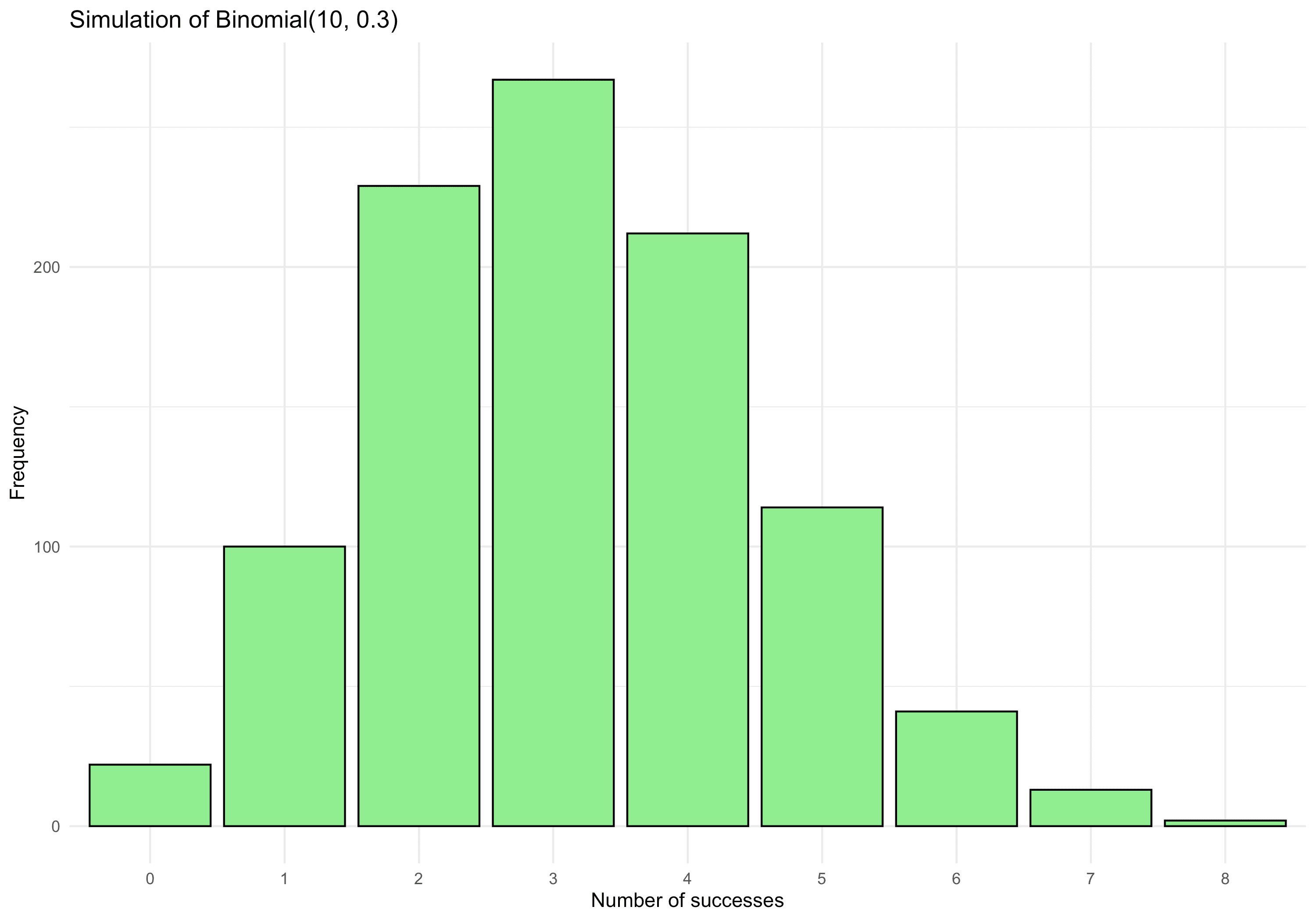
- Number of heads in
Distribution - In probability and statistics, a distribution describes how values of a random variable are spread out. It can be specified by a probability density function (pdf) for continuous variables or a probability mass function (pmf) for discrete variables.
Common examples:
- Normal distribution:
- Binomial distribution: Counts successes in
independent Bernoulli trials - Poisson distribution: Counts events in a fixed interval with known average rate
R demonstration (sampling from a normal distribution and visualising via ggplot2):
library(data.table) library(ggplot2) # Create a data.table with 1000 random N(0,1) values dt_dist <- data.table( x = rnorm(1000, mean=0, sd=1) ) # Plot a histogram ggplot(dt_dist, aes(x=x)) + geom_histogram(bins=30, colour="black", fill="skyblue") + geom_density(aes(y=..count..), colour="red", size=1) + labs( title="Histogram & Density for N(0,1)", x="Value", y="Count/Density" ) + theme_minimal()## Warning: Using `size` aesthetic for lines was deprecated in ggplot2 3.4.0. ## ℹ Please use `linewidth` instead. ## This warning is displayed once every 8 hours. ## Call `lifecycle::last_lifecycle_warnings()` to see where this warning ## was generated.## Warning: The dot-dot notation (`..count..`) was deprecated in ggplot2 3.4.0. ## ℹ Please use `after_stat(count)` instead. ## This warning is displayed once every 8 hours. ## Call `lifecycle::last_lifecycle_warnings()` to see where this warning ## was generated.
- Normal distribution:
Ellipse - An ellipse is a curve on a plane, defined as the locus of points where the sum of the distances to two fixed points (foci) is constant.
Standard form (centred at the origin):
where
and are the semi-major and semi-minor axes, respectively. R demonstration (plotting an ellipse with ggplot2):
library(data.table) library(ggplot2) # Let's parametric form: x = a*cos(t), y = b*sin(t) a <- 3 b <- 2 theta <- seq(0, 2*pi, length.out=200) dt_ellipse <- data.table( x = a*cos(theta), y = b*sin(theta) ) ggplot(dt_ellipse, aes(x=x, y=y)) + geom_path(color="blue", size=1) + coord_fixed() + labs( title="Ellipse with a=3, b=2", x="x", y="y" ) + theme_minimal()## Warning: Using `size` aesthetic for lines was deprecated in ggplot2 3.4.0. ## ℹ Please use `linewidth` instead. ## This warning is displayed once every 8 hours. ## Call `lifecycle::last_lifecycle_warnings()` to see where this warning ## was generated.
Entropy - In information theory, entropy quantifies the average amount of information contained in a random variable’s possible outcomes. For a discrete random variable
with pmf , the Shannon entropy (in bits) is: Key points:
- Entropy is maximised when all outcomes are equally likely.
- Low entropy implies outcomes are more predictable.
- It underpins coding theory, compressions, and measures of uncertainty.
R demonstration (computing entropy of a discrete distribution):
library(data.table) entropy_shannon <- function(prob_vec) { # Make sure prob_vec sums to 1 -sum(prob_vec * log2(prob_vec), na.rm=TRUE) } dt_prob <- data.table( outcome = letters[1:4], prob = c(0.1, 0.4, 0.3, 0.2) # must sum to 1 ) H <- entropy_shannon(dt_prob$prob) H## [1] 1.846439Eigenvalue - In linear algebra, an eigenvalue of a square matrix
is a scalar such that there exists a nonzero vector (the eigenvector) satisfying: Key points:
- Eigenvalues reveal important properties of linear transformations (e.g., scaling factors in certain directions).
- If
is an eigenvalue, then is an eigenvector corresponding to . - The polynomial
is the characteristic equation that yields eigenvalues.
R demonstration (finding eigenvalues of a 2x2 matrix):
library(data.table) # Create a data.table for matrix entries dtA <- data.table(a=2, b=1, c=1, d=2) A <- matrix(c(dtA$a, dtA$b, dtA$c, dtA$d), nrow=2, byrow=TRUE) A## [,1] [,2] ## [1,] 2 1 ## [2,] 1 2# Compute eigenvalues using base R eigs <- eigen(A) eigs$values## [1] 3 1eigs$vectors## [,1] [,2] ## [1,] 0.7071068 -0.7071068 ## [2,] 0.7071068 0.7071068Expectation - In probability theory, the expectation (or expected value) of a random variable
represents the long-run average outcome of after many repetitions of an experiment. For a discrete random variable:
For a continuous random variable:
where
is the probability density function. R demonstration (empirical estimation of expectation):
library(data.table) set.seed(123) # Suppose X ~ Uniform(0, 10) X_samples <- runif(10000, min=0, max=10) dtX <- data.table(X = X_samples) # Empirical mean emp_mean <- mean(dtX$X) # Theoretical expectation for Uniform(0, 10) is 5 theoretical <- 5 emp_mean## [1] 4.975494theoretical## [1] 5Field - In abstract algebra, a field is a ring in which every nonzero element has a multiplicative inverse. The real numbers
and rational numbers are classic examples of fields. Key points:
- Both addition and multiplication exist and distribute.
- Every nonzero element is invertible under multiplication.
- Foundation of much of modern mathematics (vector spaces, linear algebra).
No direct R demonstration typical.
cat("Examples: ℚ, ℝ, ℂ all form fields with standard + and *.")## Examples: ℚ, ℝ, ℂ all form fields with standard + and *.Fourier Transform - The Fourier transform is a powerful integral transform that expresses a function of time (or space) as a function of frequency. For a function
, Key points:
- Decomposes signals into sums (integrals) of sines and cosines (complex exponentials).
- Essential in signal processing, differential equations, image analysis, etc.
Discrete analogue (DFT) in R demonstration:
library(data.table) library(ggplot2) # Create a time series with two sine waves set.seed(123) n <- 256 t <- seq(0, 2*pi, length.out=n) f1 <- 1 # frequency 1 f2 <- 5 # frequency 5 signal <- sin(f1*t) + 0.5*sin(f2*t) dt_sig <- data.table( t = t, signal = signal ) # Compute discrete Fourier transform # We'll use stats::fft FT <- fft(dt_sig$signal) modulus <- Mod(FT[1:(n/2)]) # we only look at half (Nyquist) dt_dft <- data.table( freq_index = 1:(n/2), amplitude = modulus ) # Plot amplitude ggplot(dt_dft, aes(x=freq_index, y=amplitude)) + geom_line(color="blue") + labs( title="DFT amplitude spectrum", x="Frequency Index", y="Amplitude" ) + theme_minimal()
Function - A function
from a set to a set is a rule that assigns each element exactly one element . We write: Key points:
- Each input has exactly one output (well-defined).
- One of the most fundamental concepts in mathematics.
R demonstration (defining a simple function in R):
library(data.table) # A function that squares its input f <- function(x) x^2 dt_fun <- data.table( x = -3:3 ) dt_fun[, f_x := f(x)] dt_fun## x f_x ## <int> <num> ## 1: -3 9 ## 2: -2 4 ## 3: -1 1 ## 4: 0 0 ## 5: 1 1 ## 6: 2 4 ## 7: 3 9Fractal - A fractal is a geometric object that often exhibits self-similarity at various scales. Examples include the Mandelbrot set, Julia sets, and natural phenomena (coastlines, etc.).
Key traits:
- Self-similarity: Zoomed-in portions look similar to the original.
- Fractional dimension: Dimension can be non-integer.
- Often defined recursively or via iterative processes.
R demonstration (a simple iteration for the Koch snowflake boundary length, numerical only):
library(data.table) koch_iterations <- 5 dt_koch <- data.table(step = 0:koch_iterations) # Start with length 1 for the side of an equilateral triangle # Each iteration multiplies the total line length by 4/3 dt_koch[, length := (4/3)^step] dt_koch## step length ## <int> <num> ## 1: 0 1.000000 ## 2: 1 1.333333 ## 3: 2 1.777778 ## 4: 3 2.370370 ## 5: 4 3.160494 ## 6: 5 4.213992Factorial - For a positive integer
, the factorial is defined as: By convention,
. Key points:
- Factorials grow very quickly (super-exponential growth).
- Central to combinatorics:
counts the number of ways to arrange distinct objects. - Appears in formulas such as binomial coefficients
.
R demonstration (illustrating factorial growth):
library(data.table) # Let's build a small data.table of n and n! dt_fact <- data.table( n = 1:6 ) dt_fact[, factorial_n := factorial(n)] dt_fact## n factorial_n ## <int> <num> ## 1: 1 1 ## 2: 2 2 ## 3: 3 6 ## 4: 4 24 ## 5: 5 120 ## 6: 6 720Frequency - Frequency in mathematics and statistics can refer to:
- Statistical frequency: How often a value appears in a dataset.
- Periodic phenomenon: The number of cycles per unit time (e.g., in sine waves, signals).
Statistical frequency:
- Relative frequency = count of event / total observations.
- Frequency table is a basic summary in data analysis.
Periodic frequency (in signals):
- If
, then is the frequency in cycles per unit time.
R demonstration (calculating frequencies in a categorical dataset):
library(data.table) # Suppose a small categorical variable dt_freq <- data.table( category = c("A", "B", "A", "C", "B", "A", "B", "B", "C") ) # Frequency count freq_table <- dt_freq[, .N, by=category] setnames(freq_table, "N", "count") freq_table[, rel_freq := count / sum(count)] freq_table## category count rel_freq ## <char> <int> <num> ## 1: A 3 0.3333333 ## 2: B 4 0.4444444 ## 3: C 2 0.2222222Group - In abstract algebra, a group is a set
together with a binary operation satisfying: - Closure: For all
, . - Associativity:
. - Identity: There exists
such that for all . - Inverse: For each
, there exists with .
Examples:
- Integers under addition
- Nonzero real numbers under multiplication
- Symmetry groups in geometry
While direct R demonstration is less obvious, one could illustrate a finite group:
library(data.table) # Let's define a small group table: Z2 x Z2 (Klein group), with elements { (0,0), (0,1), (1,0), (1,1) } under addition mod 2 # We'll store all results in a data.table dt_group <- data.table( elem1 = c("(0,0)","(0,0)","(1,0)","(1,0)","(0,1)","(0,1)","(1,1)","(1,1)"), elem2 = c("(0,0)","(1,0)","(0,0)","(1,0)","(0,1)","(1,1)","(0,1)","(1,1)") ) # We'll define a small function that "adds" these pairs mod 2 add_mod2_pairs <- function(a, b) { # parse, e.g. "(1,0)" a_vals <- as.integer(unlist(strsplit(gsub("[()]", "", a), ","))) b_vals <- as.integer(unlist(strsplit(gsub("[()]", "", b), ","))) sum_vals <- (a_vals + b_vals) %% 2 paste0("(", sum_vals[1], ",", sum_vals[2], ")") } dt_group[, result := mapply(add_mod2_pairs, elem1, elem2)] dt_group## elem1 elem2 result ## <char> <char> <char> ## 1: (0,0) (0,0) (0,0) ## 2: (0,0) (1,0) (1,0) ## 3: (1,0) (0,0) (1,0) ## 4: (1,0) (1,0) (0,0) ## 5: (0,1) (0,1) (0,0) ## 6: (0,1) (1,1) (1,0) ## 7: (1,1) (0,1) (1,0) ## 8: (1,1) (1,1) (0,0)This small table demonstrates closure in the group. Associativity, identity, and inverses also hold, though not explicitly shown here.
- Closure: For all
Gradient - In multivariable calculus, the gradient of a scalar field
is the vector of its partial derivatives: Interpretation:
- Points in the direction of steepest ascent of
. - Magnitude represents the rate of increase in that direction.
R demonstration (numerically approximating a gradient for
at ): library(data.table) f_xy <- function(x, y) x^2 + 2*x*y numeric_grad <- function(f, x, y, h=1e-6) { df_dx <- (f(x+h, y) - f(x, y)) / h df_dy <- (f(x, y+h) - f(x, y)) / h c(df_dx, df_dy) } grad_1_2 <- numeric_grad(f_xy, 1, 2) grad_1_2 # The exact gradient is (2x + 2y, 2x). At (1,2) => (2*1 + 2*2, 2*1) => (6,2)## [1] 6.000001 2.000000- Points in the direction of steepest ascent of
Generating Function - A generating function is a formal power series whose coefficients encode information about a sequence
. For instance: Key points:
- Used extensively in combinatorics to derive closed forms or recurrences.
- Different types (ordinary, exponential) depending on the combinatorial interpretation.
Example: The ordinary generating function for the sequence
is No direct data.table example is typical here, but generating functions are used in discrete math. One might do symbolic manipulations with external packages. We can, however, illustrate partial sums numerically:
library(data.table) x_val <- 0.2 num_terms <- 10 dt_genfun <- data.table( n = 0:(num_terms-1) ) dt_genfun[, term := x_val^n] partial_sum <- dt_genfun[, sum(term)] partial_sum## [1] 1.25# Compare to closed-form 1/(1 - x_val) closed_form <- 1 / (1 - x_val) closed_form## [1] 1.25Graph - In graph theory, a graph is a set of vertices (nodes) connected by edges (links). Formally, a graph
is a pair where is the set of vertices and is the set of edges (which are pairs of vertices). Types:
- Simple vs. multigraph (multiple edges)
- Directed vs. undirected
- Weighted vs. unweighted
Applications:
- Social networks (people as nodes, relationships as edges)
- Transportation (cities as nodes, roads as edges)
- Computer science (data structures, BFS/DFS, shortest paths)
R demonstration (constructing a small graph with igraph):
library(igraph)## ## Attaching package: 'igraph'## The following objects are masked from 'package:stats': ## ## decompose, spectrum## The following object is masked from 'package:base': ## ## union# Create an undirected graph with edges g <- graph(edges=c("A","B", "B","C", "A","C", "C","D"), directed=FALSE)## Warning: `graph()` was deprecated in igraph 2.1.0. ## ℹ Please use `make_graph()` instead. ## This warning is displayed once every 8 hours. ## Call `lifecycle::last_lifecycle_warnings()` to see where this warning ## was generated.plot(g, vertex.color="lightblue", vertex.size=30)
GAN (Generative Adversarial Network) - A GAN consists of two neural networks: a generator
that produces synthetic data from random noise, and a discriminator that tries to distinguish real data from generated data. They play a minimax game: Key points:
- The generator improves to fool the discriminator, while the discriminator improves to detect fakes.
- Commonly used for image synthesis, text generation, etc.
R demonstration (Again, implementing a full GAN in R is nontrivial, but we show a minimal conceptual snippet):
library(data.table) cat("Minimal conceptual code. Usually done with torch or tensorflow in Python. We'll pseudo-code one step.\n")## Minimal conceptual code. Usually done with torch or tensorflow in Python. We'll pseudo-code one step.gen_step <- function(z, G_params) { # fwd pass to produce G(z) # ... # return synthetic data } disc_step <- function(x, D_params) { # fwd pass to produce D(x) # ... # return a probability } # Then update G_params, D_params via gradient cat("GAN training step = minimize log(1 - D(G(z))) wrt G, maximize log D(x) + log(1 - D(G(z))) wrt D.\n")## GAN training step = minimize log(1 - D(G(z))) wrt G, maximize log D(x) + log(1 - D(G(z))) wrt D.Gamma Function - The Gamma function generalises the factorial to complex (and real) arguments. For
, Key property:
for positive integers . Key points:
- Extends factorial beyond integers (e.g.,
). - Appears often in probability (Gamma distribution) and complex analysis.
R demonstration (Gamma function values):
library(data.table) # We'll evaluate Gamma at some points dt_gamma <- data.table(x = c(0.5, 1, 2, 3, 4)) dt_gamma[, gamma_x := gamma(x)] dt_gamma## x gamma_x ## <num> <num> ## 1: 0.5 1.772454 ## 2: 1.0 1.000000 ## 3: 2.0 1.000000 ## 4: 3.0 2.000000 ## 5: 4.0 6.000000- Extends factorial beyond integers (e.g.,
Homomorphism - In algebra, a homomorphism is a structure-preserving map between two algebraic structures of the same type. For instance, a group homomorphism between groups
and is a function such that:
where
is the operation in and is the operation in (see group for more on group operations). This ensures that the algebraic structure (associativity, identity, inverses) is respected.
No direct R demonstration is typical for homomorphisms, but we can quickly illustrate a trivial map:
# As a simple example: # A map from Z -> Z given by phi(x) = 2*x is a group homomorphism under addition. phi <- function(x) 2*x phi(3) # 6## [1] 6# phi(a + b) = 2*(a + b) = 2a + 2b = phi(a) + phi(b)Heaviside Step Function - The Heaviside step function, often denoted
, is defined by: Key points:
- Used in signal processing and differential equations to represent a “switch on” at
. - Sometimes defined with
or other conventions.
R demonstration:
library(data.table) H <- function(x) ifelse(x<0,0,1) test_x <- seq(-2,2,by=0.5) data.table(x=test_x, H=H(test_x))## x H ## <num> <num> ## 1: -2.0 0 ## 2: -1.5 0 ## 3: -1.0 0 ## 4: -0.5 0 ## 5: 0.0 1 ## 6: 0.5 1 ## 7: 1.0 1 ## 8: 1.5 1 ## 9: 2.0 1- Used in signal processing and differential equations to represent a “switch on” at
Hyperbola - A hyperbola is a conic section formed by the intersection of a plane and a double cone, but at a steeper angle than that of a parabola. In standard form, a hyperbola centered at the origin can be written as:
(for the east-west opening case). Hyperbolas have two branches and characteristic asymptote lines that the hyperbola approaches as
or . R demonstration (plotting a hyperbola segment in ggplot2):
library(data.table) library(ggplot2) a <- 2 b <- 1 x_vals <- seq(-5, 5, by=0.01) dt_hyp <- data.table( x = x_vals ) # For x^2/a^2 - y^2/b^2 = 1 => y^2 = (x^2/a^2 - 1)*b^2 # We only plot real solutions (where x^2/a^2 > 1) dt_hyp[, y_pos := ifelse(abs(x/a) > 1, b*sqrt((x^2/a^2) - 1), NA)]## Warning in sqrt((x^2/a^2) - 1): NaNs produceddt_hyp[, y_neg := ifelse(abs(x/a) > 1, -b*sqrt((x^2/a^2) - 1), NA)]## Warning in sqrt((x^2/a^2) - 1): NaNs producedggplot() + geom_line(aes(x=x, y=y_pos), data=dt_hyp, color="blue") + geom_line(aes(x=x, y=y_neg), data=dt_hyp, color="blue") + coord_fixed() + labs( title="Hyperbola for x^2/4 - y^2/1 = 1", x="x", y="y" ) + theme_minimal()
Hierarchical Clustering - A clustering method that builds a hierarchy of clusters either bottom-up (agglomerative) or top-down (divisive). Distances between clusters can be defined by single, complete, average linkage, etc. A dendrogram shows the merge/split hierarchy.
Algorithm (agglomerative):
- Start with each point as its own cluster.
- Merge clusters pairwise based on smallest distance until one cluster remains.
Distance metrics:
- Single linkage:
- Complete linkage:
R demonstration (using
hcluston 2D data):library(data.table) library(ggplot2) set.seed(123) n <- 50 x <- runif(n,0,5) y <- runif(n,0,5) dt_hc <- data.table(x,y) dist_mat <- dist(dt_hc[, .(x,y)]) hc <- hclust(dist_mat, method="complete") # We can cut the tree at some height to form k clusters clust <- cutree(hc, k=3) dt_hc[, cluster := factor(clust)] # Plot clusters ggplot(dt_hc, aes(x=x, y=y, color=cluster)) + geom_point(size=2) + labs(title="Hierarchical Clustering (complete linkage)", x="x", y="y") + theme_minimal()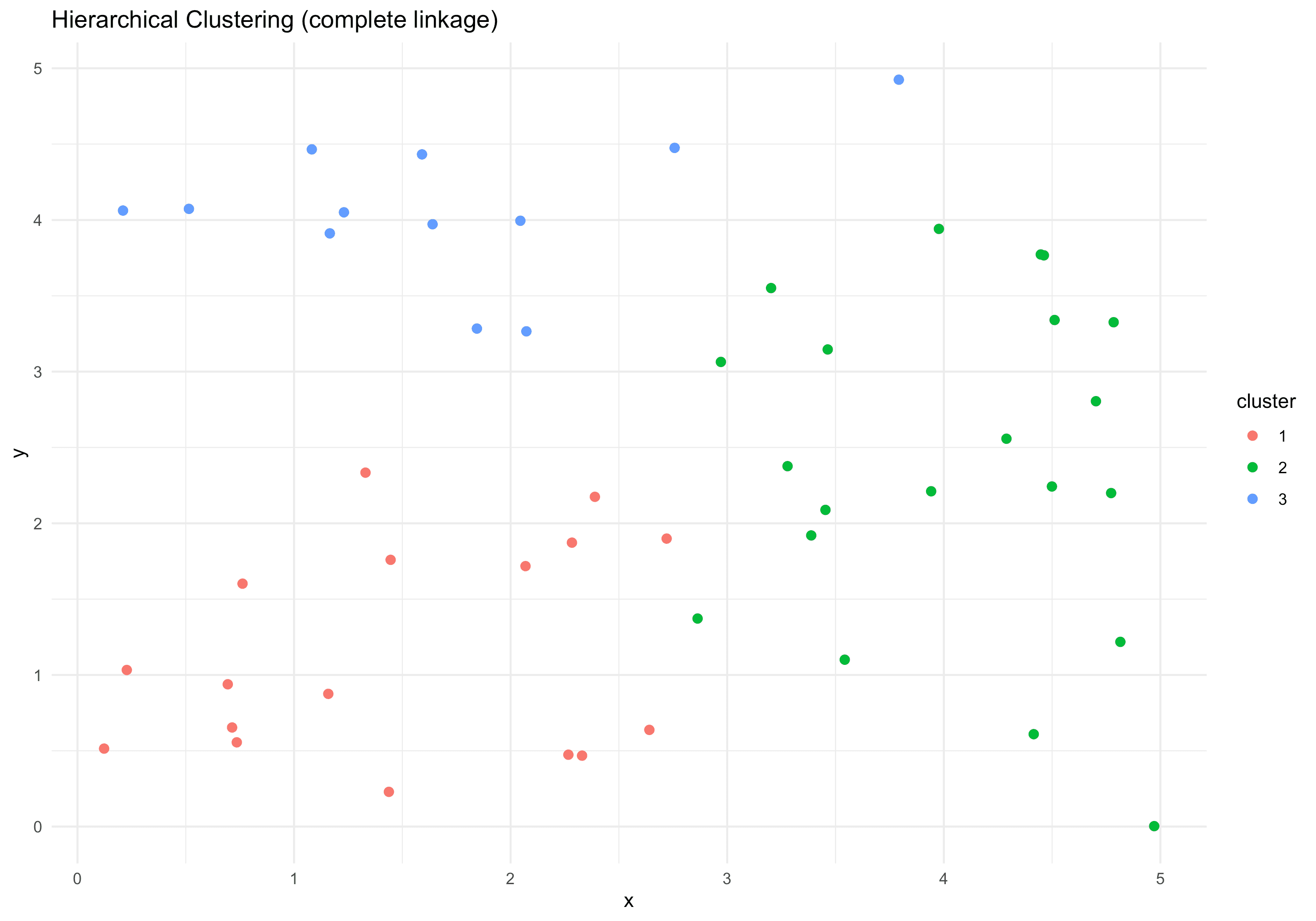
# Dendrogram plot(hc, main="Dendrogram (Complete Linkage)") rect.hclust(hc, k=3, border="red")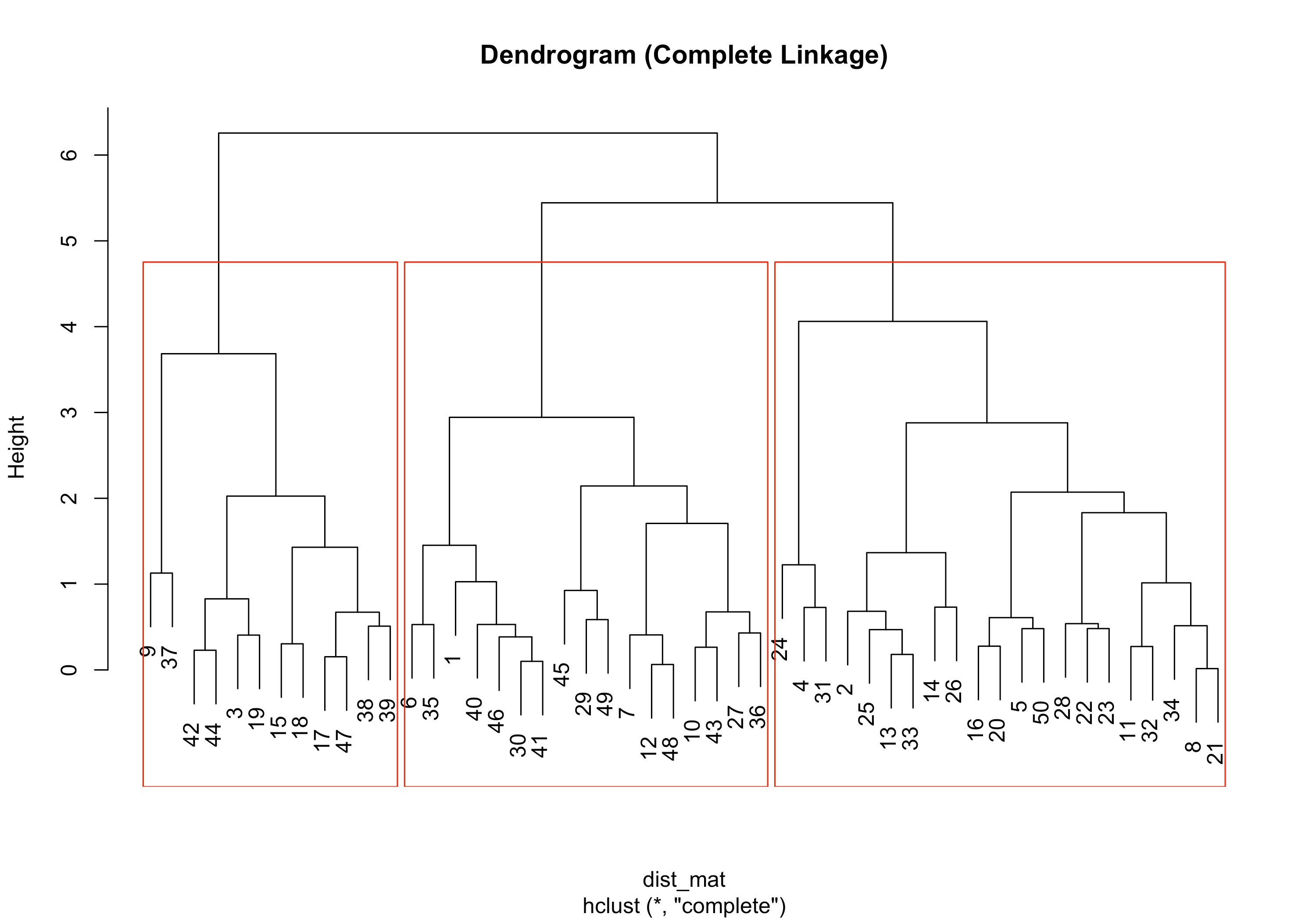
Harmonic Mean - The harmonic mean of a set of positive numbers
is defined by: - This measure is particularly useful when averaging rates or ratios.
- Compare with the arithmetic mean (the usual average), and other means (geometric, quadratic, etc.).
R demonstration (computing harmonic mean):
library(data.table) harmonic_mean <- function(x) { n <- length(x) n / sum(1/x) } dt_hm <- data.table(values = c(2, 3, 6, 6, 12)) my_hm <- harmonic_mean(dt_hm$values) my_hm## [1] 4Histogram - A histogram is a graphical representation of the distribution of numerical data. It groups data into bins (intervals) and displays the count or frequency within each bin, providing a quick visual of how values are spread.
It’s directly related to a distribution in statistics, visually summarising the frequency or relative frequency of data within specified intervals.
R demonstration (constructing a histogram):
library(data.table) library(ggplot2) set.seed(123) dt_hist <- data.table(x = rnorm(500, mean=10, sd=2)) ggplot(dt_hist, aes(x=x)) + geom_histogram(bins=30, fill="lightblue", colour="black") + labs(title="Histogram of Random Normal Data", x="Value", y="Count") + theme_minimal()
Hypothesis Testing - In statistics, hypothesis testing is a method to decide whether sample data support or refute a particular hypothesis about a population parameter or distribution.
Common steps:
- State the null hypothesis (
) and an alternative hypothesis ( ). - Choose a significance level (
) and test statistic. - Compute the p-value from sample data.
- Reject or fail to reject
based on whether the p-value is below .
R demonstration (example t-test):
library(data.table) set.seed(123) dt_ht <- data.table( groupA = rnorm(20, mean=5, sd=1), groupB = rnorm(20, mean=5.5, sd=1) ) # Let's do a two-sample t-test res <- t.test(dt_ht$groupA, dt_ht$groupB, var.equal=TRUE) res## ## Two Sample t-test ## ## data: dt_ht$groupA and dt_ht$groupB ## t = -1.0742, df = 38, p-value = 0.2895 ## alternative hypothesis: true difference in means is not equal to 0 ## 95 percent confidence interval: ## -0.8859110 0.2716729 ## sample estimates: ## mean of x mean of y ## 5.141624 5.448743- State the null hypothesis (
Induction - Mathematical induction is a proof technique used to show that a statement holds for all natural numbers. It involves two steps:
- Base Case: Prove the statement for the first natural number (often
). - Inductive Step: Assume the statement holds for some
, and then prove it holds for .
This relies on the well-ordering principle of the natural numbers.
Consider a simple example with arithmetic progressions:
- We may prove
by induction.
No complicated R demonstration is typical here, but we can at least verify sums for a few values:
library(data.table) n_vals <- 1:10 dt_ind <- data.table( n = n_vals, sum_n = sapply(n_vals, function(k) sum(1:k)), formula = n_vals*(n_vals+1)/2 ) dt_ind## n sum_n formula ## <int> <int> <num> ## 1: 1 1 1 ## 2: 2 3 3 ## 3: 3 6 6 ## 4: 4 10 10 ## 5: 5 15 15 ## 6: 6 21 21 ## 7: 7 28 28 ## 8: 8 36 36 ## 9: 9 45 45 ## 10: 10 55 55- Base Case: Prove the statement for the first natural number (often
Interval - In analysis, an interval is a connected subset of the real-number-line. Common types of intervals include:
- Open interval:
- Closed interval:
- Half-open / half-closed:
, etc.
Intervals are the building blocks of basic topology on the real line and are central in defining integrals, continuity, and other concepts of real analysis.
# Minimal R demonstration: we can define intervals simply with numeric vectors my_interval <- 0:5 # representing discrete steps from 0 to 5 my_interval## [1] 0 1 2 3 4 5- Open interval:
Integral - In calculus, an integral represents the accumulation of quantities or the area under a curve. It is the inverse operation to the derivative (by the Fundamental Theorem of Calculus).
For a function
, the definite integral from to is: Key points:
- Indefinite integral:
, where . - Riemann sums approximate integrals by partitioning the interval and summing “area slices.”
R demonstration (numeric approximation of an integral via trapezoidal rule):
library(data.table) f <- function(x) x^2 a <- 0 b <- 3 n <- 100 x_vals <- seq(a, b, length.out=n+1) dx <- (b - a)/n trapezoid <- sum((f(x_vals[-1]) + f(x_vals[-(n+1)]))/2) * dx trapezoid # approximate integral of x^2 from 0 to 3 = 9## [1] 9.00045- Indefinite integral:
Injection - In functions (set theory), an injection (or one-to-one function) is a function
such that different elements of always map to different elements of . Formally: Key points:
- No two distinct elements in
share the same image in . - Contrasts with surjection (onto) and bijection (one-to-one and onto).
R demonstration (not typical, but we can check uniqueness in a numeric map):
library(data.table) f_injective <- function(x) x^2 # for integers, watch out for collisions at +/-x x_vals <- c(-2,-1,0,1,2) f_vals <- f_injective(x_vals) data.table(x=x_vals, f=f_vals)## x f ## <num> <num> ## 1: -2 4 ## 2: -1 1 ## 3: 0 0 ## 4: 1 1 ## 5: 2 4# Notice that x^2 is not injective over all integers (f(-2)=f(2)). # But restricted to nonnegative x, it can be injective.- No two distinct elements in
Identity Matrix - In linear algebra, the identity matrix
is an square matrix with ones on the main diagonal and zeros elsewhere: Key points:
serves as the multiplicative identity for matrices: . - Its determinant is 1 for all
. - Invertible matrices always have an identity matrix (the “unit” of their multiplicative structure).
R demonstration (creating identity matrices):
library(data.table) I2 <- diag(2) I3 <- diag(3) I2## [,1] [,2] ## [1,] 1 0 ## [2,] 0 1I3## [,1] [,2] [,3] ## [1,] 1 0 0 ## [2,] 0 1 0 ## [3,] 0 0 1Intersection - In set theory, the intersection of two sets
and is the set of elements that belong to both and . Symbolically: - Compare this with the union
, which combines all elements in either or . - The empty set
results if and share no elements.
No special R demonstration is typically needed, but we can illustrate a basic example using sets as vectors:
A <- c(1, 2, 3, 4) B <- c(3, 4, 5, 6) intersect(A, B) # yields 3,4## [1] 3 4- Compare this with the union
Jensen's Inequality - In analysis, Jensen’s inequality states that for a convex function
and a random variable , If
is concave, the inequality reverses. This has deep implications in expectation and probability theory. R demonstration (empirical illustration):
library(data.table) set.seed(123) X <- runif(1000, min=0, max=2) # random draws in [0,2] phi <- function(x) x^2 # a convex function mean_X <- mean(X) lhs <- phi(mean_X) rhs <- mean(phi(X)) lhs## [1] 0.9891408rhs## [1] 1.319398# Typically: lhs <= rhs (Jensen's inequality for convex phi)Jacobian - In multivariable calculus, the Jacobian of a vector function
is thematrix of all first-order partial derivatives: - The determinant of this matrix (if
) is often used in change-of-variable formulas. - It generalises the concept of the gradient (when
).
R demonstration (numerical approximation of a Jacobian):
library(data.table) f_xy <- function(x, y) c(x^2 + 3*y, 2*x + y^2) approx_jacobian <- function(f, x, y, h=1e-6) { # f should return a vector c(f1, f2, ...) # We'll approximate partial derivatives w.r.t x and y. f_at_xy <- f(x, y) # partial w.r.t x f_at_xplus <- f(x + h, y) df_dx <- (f_at_xplus - f_at_xy) / h # partial w.r.t y f_at_yplus <- f(x, y + h) df_dy <- (f_at_yplus - f_at_xy) / h rbind(df_dx, df_dy) } approx_jacobian(f_xy, 1, 2)## [,1] [,2] ## df_dx 2.000001 2.000000 ## df_dy 3.000000 4.000001- The determinant of this matrix (if
Julia Set - In complex dynamics, a Julia set is the boundary of points in the complex plane describing the behaviour of a complex function, often associated with the iteration of polynomials like
. Julia sets are typical examples of a fractal. Key points:
- For each complex parameter
, there is a distinct Julia set. - The set often exhibits self-similarity and intricate boundaries.
R demonstration (simple iteration to classify points):
library(data.table) library(ggplot2) # We'll do a basic "escape-time" iteration for z^2 + c, with c = -0.8 + 0.156i c_val <- complex(real=-0.8, imaginary=0.156) n <- 400 x_seq <- seq(-1.5, 1.5, length.out=n) y_seq <- seq(-1.5, 1.5, length.out=n) max_iter <- 50 threshold <- 2 res <- data.table() for (ix in seq_along(x_seq)) { for (iy in seq_along(y_seq)) { z <- complex(real=x_seq[ix], imaginary=y_seq[iy]) iter <- 0 while(Mod(z) < threshold && iter < max_iter) { z <- z*z + c_val iter <- iter + 1 } res <- rbind( res, data.table( x = x_seq[ix], y = y_seq[iy], iteration = iter ) ) } } ggplot(res, aes(x=x, y=y, color=iteration)) + geom_point(shape=15, size=1) + scale_color_viridis_c() + coord_fixed() + labs( title="Simple Julia Set (z^2 + c)", x="Re(z)", y="Im(z)" ) + theme_minimal()
- For each complex parameter
Jordan Normal Form - In linear algebra, the Jordan normal form (or Jordan canonical form) of a matrix is a block diagonal matrix with Jordan blocks, each corresponding to an eigenvalue.
A Jordan block for an eigenvalue
looks like: The Jordan form classifies matrices up to similarity transformations and is critical in solving systems of linear differential equations and more.
R demonstration (no built-in base R function to compute Jordan form, but we can show a small example):
library(data.table) # Usually, packages like 'jord' or 'expm' might help. # We'll just illustrate a 2x2 Jordan block for eigenvalue 3: J <- matrix(c(3,1,0,3), 2, 2, byrow=TRUE) J## [,1] [,2] ## [1,] 3 1 ## [2,] 0 3Joint Distribution - In statistics, a joint distribution describes the probability distribution of two or more random variables simultaneously. If
and are two random variables: - Joint pmf (discrete case):
- Joint pdf (continuous case):
It extends the idea of a single-variable distribution to multiple dimensions.
R demonstration (bivariate normal sampling):
library(MASS) # for mvrnorm library(data.table) library(ggplot2) Sigma <- matrix(c(1, 0.5, 0.5, 1), 2, 2) # Cov matrix mu <- c(0, 0) set.seed(123) dt_joint <- data.table( mvrnorm(n=1000, mu=mu, Sigma=Sigma) ) setnames(dt_joint, c("V1","V2"), c("X","Y")) # Plot joint distribution via scatter plot ggplot(dt_joint, aes(x=X, y=Y)) + geom_point(alpha=0.5) + labs( title="Bivariate Normal Scatter", x="X", y="Y" ) + theme_minimal()
- Joint pmf (discrete case):
Kolmogorov Complexity - In algorithmic information theory, Kolmogorov complexity of a string is the length of the shortest description (program) that can produce that string on a universal computer (like a universal Turing machine).
Key Points:
- Measures the “information content” of a string.
- Uncomputable in the general case (no algorithm can compute the exact Kolmogorov complexity for every string).
- Often used to reason about randomness and compressibility.
No direct R demonstration is typical, as computing or estimating Kolmogorov complexity is a deep problem, but we can reason about approximate compression lengths with standard compressors.
Kruskal's Algorithm - In graph theory, Kruskal's algorithm finds a minimum spanning tree (MST) of a weighted graph by:
- Sorting edges in order of increasing weight.
- Adding edges one by one to the MST, provided they do not form a cycle.
- Repeating until all vertices are connected or edges are exhausted.
This greedy approach ensures an MST if the graph is connected.
R demonstration (a small example with igraph):
library(igraph)## ## Attaching package: 'igraph'## The following objects are masked from 'package:stats': ## ## decompose, spectrum## The following object is masked from 'package:base': ## ## union# Create a weighted graph g <- graph(edges=c("A","B","B","C","A","C","C","D","B","D"), directed=FALSE)## Warning: `graph()` was deprecated in igraph 2.1.0. ## ℹ Please use `make_graph()` instead. ## This warning is displayed once every 8 hours. ## Call `lifecycle::last_lifecycle_warnings()` to see where this warning ## was generated.E(g)$weight <- c(2, 4, 5, 1, 3) # just some weights # Use built-in MST function that uses Kruskal internally mst_g <- mst(g) mst_g## IGRAPH d1aa2b3 UNW- 4 3 -- ## + attr: name (v/c), weight (e/n) ## + edges from d1aa2b3 (vertex names): ## [1] A--B C--D B--D# Let's plot plot(mst_g, vertex.color="lightblue", vertex.size=30, edge.label=E(mst_g)$weight)
Kernel - In linear algebra, the kernel (or null space) of a linear map
is the set of all vectors such that . Symbolically, - If
is given by a matrix , then . - The rank-nullity theorem links the dimension of the kernel with the dimension of the image.
R demonstration (finding the kernel of a matrix):
library(data.table) A <- matrix(c(1,2,3, 2,4,6, 1,1,2), nrow=3, byrow=TRUE) # We can find the null space using MASS::Null library(MASS) kerA <- Null(A) # basis for the kernel kerA## [,1] ## [1,] -8.944272e-01 ## [2,] 4.472136e-01 ## [3,] -1.024712e-15- If
K-Nearest Neighbors (KNN) - A KNN classifier (or regressor) predicts the label (or value) of a new point
by looking at the k closest points (in some distance metric) in the training set. For classification, it uses a majority vote among neighbors; for regression, it averages the neighbor values. Mathematical form (for classification):
where
is the set of k nearest neighbors under a chosen distance (often Euclidean). R demonstration (using
class::knnfor classification):library(class) library(data.table) library(ggplot2) set.seed(123) n <- 100 x1 <- runif(n, 0, 5) x2 <- runif(n, 0, 5) y <- ifelse(x1 + x2 + rnorm(n) > 5, "A","B") dt_knn <- data.table(x1=x1, x2=x2, y=as.factor(y)) # We'll do a train/test split train_idx <- sample(1:n, size=70) train <- dt_knn[train_idx] test <- dt_knn[-train_idx] train_x <- as.matrix(train[, .(x1,x2)]) train_y <- train$y test_x <- as.matrix(test[, .(x1,x2)]) true_y <- test$y pred_knn <- knn(train_x, test_x, cl=train_y, k=3) accuracy <- mean(pred_knn == true_y) accuracy## [1] 0.8333333# Plot classification boundary grid_x1 <- seq(0,5, by=0.1) grid_x2 <- seq(0,5, by=0.1) grid_data <- data.table(expand.grid(x1=grid_x1, x2=grid_x2)) grid_mat <- as.matrix(grid_data[,.(x1,x2)]) grid_data[, pred := knn(train_x, grid_mat, cl=train_y, k=3)] ggplot() + geom_tile(data=grid_data, aes(x=x1, y=x2, fill=pred), alpha=0.4) + geom_point(data=dt_knn, aes(x=x1, y=x2, color=y), size=2) + scale_fill_manual(values=c("A"="lightblue","B"="salmon")) + scale_color_manual(values=c("A"="blue","B"="red")) + labs(title="K-Nearest Neighbors (k=3)", x="x1", y="x2") + theme_minimal()
K-means - In cluster analysis, k-means is an algorithm that partitions
observations into clusters. Each observation belongs to the cluster with the nearest mean (cluster centre). Algorithm Outline:
- Choose
initial centroids. - Assign each data point to its nearest centroid.
- Recompute centroids as the mean of points in each cluster.
- Repeat steps 2-3 until assignments stabilize or a maximum iteration count is reached.
K-means often assumes data in a continuous space and can leverage knowledge of the distribution of points to identify cluster structure.
R demonstration (basic example):
library(data.table) library(ggplot2) set.seed(123) dt_data <- data.table( x = rnorm(50, 5, 1), y = rnorm(50, 2, 1) ) # Add another cluster dt_data2 <- data.table( x = rnorm(50, 10, 1), y = rnorm(50, 7, 1) ) dt_full <- rbind(dt_data, dt_data2) # k-means with 2 clusters res_km <- kmeans(dt_full[, .(x, y)], centers=2) dt_full[, cluster := factor(res_km$cluster)] ggplot(dt_full, aes(x=x, y=y, color=cluster)) + geom_point() + labs( title="k-means Clustering (k=2)", x="X", y="Y" ) + theme_minimal()
- Choose
Kurtosis - In statistics, kurtosis measures the “tailedness” of a distribution. The standard formula for sample kurtosis (excess kurtosis) is often:
- High kurtosis: heavy tails, outliers are more frequent.
- Low kurtosis: light tails, fewer extreme outliers (relative to a normal distribution).
R demonstration:
library(data.table) library(e1071) # for kurtosis function set.seed(123) dt_kurt <- data.table( normal = rnorm(500, mean=0, sd=1), heavy_tail = rt(500, df=3) # t-dist with df=3, heavier tails ) k_norm <- e1071::kurtosis(dt_kurt$normal) k_heavy <- e1071::kurtosis(dt_kurt$heavy_tail) k_norm## [1] -0.05820728k_heavy## [1] 7.802004Laplace Transform - In calculus, the Laplace transform of a function
(for ) is defined by the integral: assuming the integral converges.
Key points:
- Simplifies solving ordinary differential equations by converting them into algebraic equations in the
-domain. - Inverse Laplace transform recovers
from .
R demonstration (no base R function for Laplace transforms, but we can do numeric approximations or use external packages. We show a naive numeric approach for a simple function
): library(data.table) f <- function(t) exp(-t) laplace_numeric <- function(f, s, upper=10, n=1000) { # naive numerical approach t_vals <- seq(0, upper, length.out=n) dt <- (upper - 0)/n sum( exp(-s * t_vals) * f(t_vals) ) * dt } s_test <- 2 approx_LT <- laplace_numeric(f, s_test, upper=10) approx_LT## [1] 0.338025# The exact Laplace transform of e^{-t} is 1/(s+1). For s=2 => 1/3 ~ 0.3333- Simplifies solving ordinary differential equations by converting them into algebraic equations in the
Laplacian - In multivariable calculus, the Laplacian of a scalar function
is denoted by or , and is defined as: - In 2D:
. - In 3D:
. - The concept generalises to higher dimension.
- The Laplacian is crucial in PDEs like the heat equation and wave equation.
No direct R built-in for second partial derivatives numerically, but we can approximate:
library(data.table) f_xy <- function(x, y) x^2 + y^2 laplacian_approx <- function(f, x, y, h=1e-4) { # second partial w.r.t x f_xph <- f(x+h, y); f_xmh <- f(x-h, y); f_xyc <- f(x, y) d2f_dx2 <- (f_xph - 2*f_xyc + f_xmh)/(h^2) # second partial w.r.t y f_yph <- f(x, y+h); f_ymh <- f(x, y-h) d2f_dy2 <- (f_yph - 2*f_xyc + f_ymh)/(h^2) d2f_dx2 + d2f_dy2 } laplacian_approx(f_xy, 2, 3)## [1] 4# For f(x,y)= x^2 + y^2, exact Laplacian = 2 + 2 = 4- In 2D:
L'Hôpital's Rule - In calculus, L'Hôpital's rule is a result for evaluating certain indeterminate forms of limit expressions. If
produces indeterminate forms like
or , then (under certain conditions involving differentiability and continuity): provided the latter limit exists. It relies on the concept of the derivative.
Simple R demonstration (symbolic approach would be used in a CAS, but we can do numeric checks):
library(data.table) f <- function(x) x^2 - 1 g <- function(x) x - 1 # Evaluate near x=1 to see 0/0 x_vals <- seq(0.9, 1.1, by=0.01) dt_lhop <- data.table( x = x_vals, f_x = f(x_vals), g_x = g(x_vals), ratio = f(x_vals)/g(x_vals) ) head(dt_lhop)## x f_x g_x ratio ## <num> <num> <num> <num> ## 1: 0.90 -0.1900 -0.10 1.90 ## 2: 0.91 -0.1719 -0.09 1.91 ## 3: 0.92 -0.1536 -0.08 1.92 ## 4: 0.93 -0.1351 -0.07 1.93 ## 5: 0.94 -0.1164 -0.06 1.94 ## 6: 0.95 -0.0975 -0.05 1.95We can see the ratio near x=1 is close to the ratio of derivatives at that point:
- f'(x) = 2x
- g'(x) = 1 So at x=1, ratio ~ 2(1)/1 = 2.
Limit - In calculus, a limit describes the value that a function (or sequence) “approaches” as the input (or index) moves toward some point. For a function
: means that
can be made arbitrarily close to by taking sufficiently close to . Key role in:
- Defining the derivative:
. - Defining continuity and integrals.
R demonstration (numeric approximation of a limit at a point):
library(data.table) f <- function(x) (x^2 - 1)/(x - 1) # Indeterminate at x=1, but simplifies to x+1 x_vals <- seq(0.9, 1.1, by=0.01) dt_lim <- data.table( x = x_vals, f_x = f(x_vals) ) dt_lim## x f_x ## <num> <num> ## 1: 0.90 1.90 ## 2: 0.91 1.91 ## 3: 0.92 1.92 ## 4: 0.93 1.93 ## 5: 0.94 1.94 ## 6: 0.95 1.95 ## 7: 0.96 1.96 ## 8: 0.97 1.97 ## 9: 0.98 1.98 ## 10: 0.99 1.99 ## 11: 1.00 NaN ## 12: 1.01 2.01 ## 13: 1.02 2.02 ## 14: 1.03 2.03 ## 15: 1.04 2.04 ## 16: 1.05 2.05 ## 17: 1.06 2.06 ## 18: 1.07 2.07 ## 19: 1.08 2.08 ## 20: 1.09 2.09 ## 21: 1.10 2.10 ## x f_x# As x -> 1, f(x)-> 2.- Defining the derivative:
LDA (Linear Discriminant Analysis) - A linear discriminant analysis technique for classification which finds a linear combination of features that best separates classes. It aims to maximise between-class variance over within-class variance.
Mathematical objective: Given classes
, let be their means and the pooled covariance (assuming classes share the same covariance). We want to find a projection vector solving: where
is between-class scatter, is within-class scatter.
R demonstration (using
MASS::ldaon synthetic data):library(MASS) library(data.table) library(ggplot2) set.seed(123) n <- 50 x1_class1 <- rnorm(n, mean=2, sd=1) x2_class1 <- rnorm(n, mean=2, sd=1) x1_class2 <- rnorm(n, mean=-2, sd=1) x2_class2 <- rnorm(n, mean=-2, sd=1) dt_lda_ex <- data.table( x1 = c(x1_class1, x1_class2), x2 = c(x2_class1, x2_class2), y = factor(c(rep("Class1", n), rep("Class2", n))) ) fit_lda <- lda(y ~ x1 + x2, data=dt_lda_ex) fit_lda## Call: ## lda(y ~ x1 + x2, data = dt_lda_ex) ## ## Prior probabilities of groups: ## Class1 Class2 ## 0.5 0.5 ## ## Group means: ## x1 x2 ## Class1 2.034404 2.146408 ## Class2 -2.253900 -1.961193 ## ## Coefficients of linear discriminants: ## LD1 ## x1 -0.7461484 ## x2 -0.7780657# Project data onto LD1 proj <- predict(fit_lda) dt_proj <- cbind(dt_lda_ex, LD1=proj$x[,1]) ggplot(dt_proj, aes(x=LD1, fill=y)) + geom_histogram(alpha=0.6, position="identity") + labs(title="LDA Projection onto LD1", x="LD1", y="Count") + theme_minimal()## `stat_bin()` using `bins = 30`. Pick better value with `binwidth`.
Linear Regression - In machine learning and statistics, linear regression models the relationship between a scalar response
and one or more explanatory variables (features) by fitting a linear equation: Key points:
- Least squares estimates the coefficients
by minimising the sum of squared residuals. - The fitted line (or hyperplane in multiple dimensions) can be used for prediction and inference.
Mathematical formula: If we have data
for i=1..m in a single-feature scenario, the sum of squared errors is: We find
that minimise this sum. R demonstration (fitting a simple linear regression using base R):
library(data.table) set.seed(123) n <- 20 x <- runif(n, min=0, max=10) y <- 3 + 2*x + rnorm(n, mean=0, sd=2) # "true" slope=2, intercept=3 dt_lr <- data.table(x=x, y=y) fit <- lm(y ~ x, data=dt_lr) summary(fit)## ## Call: ## lm(formula = y ~ x, data = dt_lr) ## ## Residuals: ## Min 1Q Median 3Q Max ## -2.8189 -1.2640 -0.1737 1.3732 3.7852 ## ## Coefficients: ## Estimate Std. Error t value Pr(>|t|) ## (Intercept) 4.2326 0.8766 4.828 0.000135 *** ## x 1.7370 0.1392 12.481 2.67e-10 *** ## --- ## Signif. codes: 0 '***' 0.001 '**' 0.01 '*' 0.05 '.' 0.1 ' ' 1 ## ## Residual standard error: 1.902 on 18 degrees of freedom ## Multiple R-squared: 0.8964, Adjusted R-squared: 0.8907 ## F-statistic: 155.8 on 1 and 18 DF, p-value: 2.673e-10# Plot plot(y ~ x, data=dt_lr, pch=19, main="Linear Regression Demo") abline(fit, col="red", lwd=2)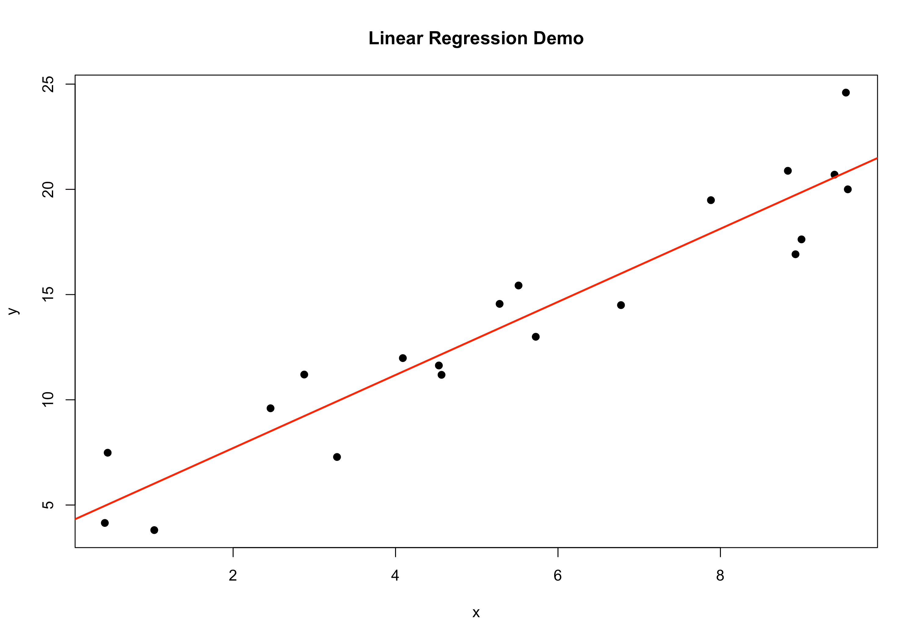
- Least squares estimates the coefficients
LLM (Large Language Model) - A large language model is typically a Transformer-based or similarly advanced architecture with billions (or more) of parameters, trained on massive text corpora to generate coherent text or perform NLP tasks.
Key points:
- Uses self-attention to handle long contexts.
- Learns complex linguistic structures, can generate next tokens based on context.
Mathematical gist: At each token step, an LLM computes a probability distribution over the vocabulary:
where
is the hidden representation after attention layers. R demonstration (We can show a mini example of text generation with
keras, but typically giant LLM training isn't feasible in R. We'll do conceptual snippet):# Conceptual only: library(data.table) cat("Training an LLM is typically done in Python with large GPU clusters.\nWe'll do a small toy example with a simple RNN or minimal next-token model.")## Training an LLM is typically done in Python with large GPU clusters. ## We'll do a small toy example with a simple RNN or minimal next-token model.Likelihood - In statistics, the likelihood function measures how well a given model parameter explains observed data. It’s similar to a distribution but viewed from the parameter’s perspective:
- For data
and parameter , the likelihood is often expressed as , the probability of observing given .
Key points:
- Maximum likelihood estimation chooses
that maximises . - Log-likelihood is commonly used for convenience:
.
R demonstration (fitting a simple normal likelihood):
library(data.table) set.seed(123) x_data <- rnorm(50, mean=5, sd=2) lik_fun <- function(mu, sigma, x) { # Normal pdf for each x, product as likelihood # i.e. prod(dnorm(x, mean=mu, sd=sigma)) # We'll return negative log-likelihood for convenience -sum(dnorm(x, mean=mu, sd=sigma, log=TRUE)) } # We'll do a quick grid search mu_seq <- seq(4, 6, by=0.1) sigma_seq <- seq(1, 3, by=0.1) res <- data.table() for(m in mu_seq) { for(s in sigma_seq) { nll <- lik_fun(m, s, x_data) res <- rbind(res, data.table(mu=m, sigma=s, nll=nll)) } } res_min <- res[which.min(nll)] res_min## mu sigma nll ## <num> <num> <num> ## 1: 5.1 1.8 101.2725- For data
Monoid - In abstract algebra, a monoid is a semigroup with an identity element. Specifically, a set
with an associative binary operation and an identity element so: - Associativity:
for all . - Identity:
for all .
Key points:
- A group is a monoid where every element also has an inverse.
- Examples: Natural numbers under addition with identity 0, strings under concatenation with identity "" (empty string).
No direct R demonstration typical, but we can show a small "string monoid":
library(data.table) str_monoid_op <- function(a,b) paste0(a,b) # concatenation e <- "" # identity # Check associativity on a small example a<-"cat"; b<-"fish"; c<-"food" assoc_left <- str_monoid_op(str_monoid_op(a,b), c) assoc_right <- str_monoid_op(a, str_monoid_op(b,c)) data.table(assoc_left, assoc_right)## assoc_left assoc_right ## <char> <char> ## 1: catfishfood catfishfood- Associativity:
Matrix - A matrix is a rectangular array of numbers (or more abstract objects) arranged in rows and columns. Matrices are fundamental in determinant calculations, linear transformations, and a variety of applications:
Key operations:
- Addition and scalar multiplication (element-wise).
- Matrix multiplication.
- Transposition and inversion (if square and invertible).
R demonstration (basic matrix creation and operations):
library(data.table) A <- matrix(c(1,2,3,4,5,6), nrow=2, byrow=TRUE) B <- matrix(c(10,20,30,40,50,60), nrow=2, byrow=TRUE) A_plus_B <- A + B A_times_B <- A %*% t(B) # 2x3 %*% 3x2 => 2x2 A_plus_B## [,1] [,2] [,3] ## [1,] 11 22 33 ## [2,] 44 55 66A_times_B## [,1] [,2] ## [1,] 140 320 ## [2,] 320 770Markov Chain - In probability, a Markov chain is a stochastic-process with the Markov property: the next state depends only on the current state, not the history. Formally:
Key points:
- Transition probabilities can be arranged in a matrix for finite state spaces.
- Widely used in queueing, random walks, genetics, finance.
R demonstration (a simple Markov chain simulation):
library(data.table) # Transition matrix for states A,B P <- matrix(c(0.7, 0.3, 0.4, 0.6), nrow=2, byrow=TRUE) rownames(P) <- colnames(P) <- c("A","B") simulate_markov <- function(P, n=10, start="A") { states <- rownames(P) chain <- character(n) chain[1] <- start for(i in 2:n) { current <- chain[i-1] idx <- which(states==current) chain[i] <- sample(states, 1, prob=P[idx,]) } chain } chain_res <- simulate_markov(P, n=15, start="A") chain_res## [1] "A" "A" "A" "B" "B" "B" "A" "B" "A" "A" "B" "A" "A" "A" "A"Mutually Exclusive Events - In probability, two events
and are mutually exclusive (or disjoint) if they cannot happen simultaneously: In other words,
. The union of mutually exclusive events has a probability that’s just the sum of their individual probabilities: since
and never overlap. R demonstration: no direct R function, but we can illustrate logic:
# Suppose events are flipping a coin: # A = heads, B = tails # A and B are mutually exclusive. # We can do a small simulation set.seed(123) flips <- sample(c("H","T"), size=100, replace=TRUE) mean(flips == "H") # approximate P(A)## [1] 0.57mean(flips == "T") # approximate P(B)## [1] 0.43# Overlap: none, because a single flip can't be both H and TMean - In statistics, the mean (or average) of a set of values
is: This is the arithmetic mean. Compare to the harmonic-mean or geometric mean for other contexts. The mean is often used to summarise a distribution.
R demonstration:
library(data.table) dt_values <- data.table(val = c(2,3,5,7,11)) mean_val <- mean(dt_values$val) mean_val## [1] 5.6Median - In statistics, the median is the value separating the higher half from the lower half of a distribution. For an ordered dataset of size
: - If
is odd, the median is the middle value. - If
is even, the median is the average of the two middle values.
R demonstration:
library(data.table) dt_vals <- data.table(val = c(2,3,7,9,11)) med_val <- median(dt_vals$val) med_val## [1] 7- If
Mode - In statistics, the mode is the most frequently occurring value in a distribution. Some distributions (e.g., uniform) may have multiple modes (or no strong mode) if all values are equally likely.
R demonstration (custom function):
library(data.table) mode_fn <- function(x) { # returns the value(s) with highest frequency tab <- table(x) freq_max <- max(tab) as.numeric(names(tab)[tab == freq_max]) } dt_data <- data.table(vals = c(1,2,2,3,2,5,5,5)) mode_fn(dt_data$vals)## [1] 2 5Manifold - In topology and differential geometry, a manifold is a topological-space that locally resembles Euclidean space. Formally, an
-dimensional manifold is a space where every point has a neighbourhood homeomorphic to . Key points:
- The concept of dimension is central: a 2D manifold locally looks like a plane, a 3D manifold like space, etc.
- Smooth manifolds allow calculus-like operations on them.
No direct R demonstration, but we can illustrate how to store a “chart” or local coordinate system conceptually:
library(data.table) cat("Manifolds are an advanced concept. In R, we'd handle geometry libraries for numeric solutions.")## Manifolds are an advanced concept. In R, we'd handle geometry libraries for numeric solutions.Nested Radical - A nested radical is an expression containing radicals (square roots, etc.) inside other radicals, for example:
Such expressions sometimes simplify to closed-forms. A famous example is:
Though symbolic manipulation is more typical than numeric for these. Minimal R demonstration here:
# We could approximate a short nested radical numerically: nested_radical_approx <- function(n) { # approximate: sqrt(1 + 2*sqrt(1 + 3*sqrt(1+... up to n steps # This is more a demonstration than a standard function val <- 0 for(k in seq(n, 2, by=-1)) { val <- sqrt(1 + k*val) } sqrt(1 + 2*val) # final } nested_radical_approx(5)## [1] 2.473795Number Line - The number line (real line) is a straight line on which every real number corresponds to a unique point. Basic structures like an interval are subsets of the number line:
- Negative numbers extend to the left, positive numbers to the right.
- Zero is typically placed at the origin.
No direct R demonstration is typical, but we can illustrate numeric representations:
library(data.table) vals <- seq(-3, 3, by=1) vals## [1] -3 -2 -1 0 1 2 3Non-Euclidean Geometry - In geometry, non-Euclidean geometry refers to either hyperbolic or elliptic geometry (or others) that reject or modify Euclid’s fifth postulate (the parallel postulate).
Key points:
- Hyperbolic geometry: infinite lines diverge more rapidly, sums of angles in triangles are < 180°.
- Elliptic geometry: lines “curve,” angles in triangles sum to > 180°.
No standard R demonstration, but we might explore transformations or plots for illustrative geometry.
# No direct numeric example, but let's just place a note: cat("No direct numeric example for non-Euclidean geometry in base R. Consider specialized geometry packages or external tools.")## No direct numeric example for non-Euclidean geometry in base R. Consider specialized geometry packages or external tools.Naive Bayes - In machine learning, Naive Bayes is a probabilistic classifier applying Bayes' theorem with a “naive” (independence) assumption among features given the class. For a class
and features : Key points:
- Independence assumption simplifies computation of
. - Effective in text classification (bag-of-words assumption).
R demonstration (using
e1071::naiveBayeson synthetic data):library(e1071) library(data.table) library(ggplot2) set.seed(123) n <- 100 x1 <- rnorm(n, mean=2, sd=1) x2 <- rnorm(n, mean=-1, sd=1) cl1 <- data.table(x1, x2, y="Class1") x1 <- rnorm(n, mean=-2, sd=1) x2 <- rnorm(n, mean=2, sd=1) cl2 <- data.table(x1, x2, y="Class2") dt_nb <- rbind(cl1, cl2) fit_nb <- naiveBayes(y ~ x1 + x2, data=dt_nb) fit_nb## ## Naive Bayes Classifier for Discrete Predictors ## ## Call: ## naiveBayes.default(x = X, y = Y, laplace = laplace) ## ## A-priori probabilities: ## Y ## Class1 Class2 ## 0.5 0.5 ## ## Conditional probabilities: ## x1 ## Y [,1] [,2] ## Class1 2.090406 0.9128159 ## Class2 -1.879535 0.9498790 ## ## x2 ## Y [,1] [,2] ## Class1 -1.107547 0.9669866 ## Class2 1.963777 1.0387812# Predict grid_x1 <- seq(-5,5, by=0.2) grid_x2 <- seq(-5,5, by=0.2) grid_data <- data.table(expand.grid(x1=grid_x1, x2=grid_x2)) grid_data[, pred := predict(fit_nb, newdata=.SD)] ggplot() + geom_tile(data=grid_data, aes(x=x1, y=x2, fill=pred), alpha=0.4) + geom_point(data=dt_nb, aes(x=x1, y=x2, color=y), size=2) + scale_fill_manual(values=c("Class1"="lightblue","Class2"="salmon")) + scale_color_manual(values=c("Class1"="blue","Class2"="red")) + labs(title="Naive Bayes Classification", x="x1", y="x2") + theme_minimal()
- Independence assumption simplifies computation of
Neural Network - In machine learning, a neural network is a collection of connected units (neurons) arranged in layers. Each neuron computes a weighted sum of inputs, applies an activation function
, and passes the result to the next layer. Key points:
- A typical feed-forward network with one hidden layer might compute: '60196' z_1^1 = \sigma( W_1 x + b_1), \quad z_2^2 = \sigma( W_2 z_1^1 + b_2 ), '60196'
- Training uses gradient-based optimisation (see gradient) (e.g., backpropagation) to adjust weights.
R demonstration (a small neural network using
nnetpackage):library(data.table) library(nnet) set.seed(123) n <- 50 x <- runif(n, min=0, max=2*pi) y <- sin(x) + rnorm(n, sd=0.1) dt_nn <- data.table(x=x, y=y) # Fit a small single-hidden-layer neural network fit_nn <- nnet(y ~ x, data=dt_nn, size=5, linout=TRUE, trace=FALSE) # Predictions newx <- seq(0,2*pi,length.out=100) pred_y <- predict(fit_nn, newdata=data.table(x=newx)) plot(dt_nn, dt_nn, main="Neural Network Demo", pch=19) lines(newx, sin(newx), col="blue", lwd=2, lty=2) # true function lines(newx, pred_y, col="red", lwd=2) # NN approximation
Normal Distribution - In statistics, the normal distribution (or Gaussian) is a continuous probability distribution with probability density function:
where '56956'\mu'56956' is the mean and '56956'\sigma^2'56956' is the variance.
Key points:
- Symmetric, bell-shaped curve.
- Many natural phenomena approximate normality by Central Limit Theorem arguments.
R demonstration:
library(data.table) library(ggplot2) set.seed(123) dt_norm <- data.table(x = rnorm(1000, mean=5, sd=2)) ggplot(dt_norm, aes(x=x)) + geom_histogram(bins=30, fill="lightblue", color="black", aes(y=..density..)) + geom_density(color="red", size=1) + labs( title="Normal Distribution Example", x="Value", y="Density" ) + theme_minimal()## Warning: Using `size` aesthetic for lines was deprecated in ggplot2 3.4.0. ## ℹ Please use `linewidth` instead. ## This warning is displayed once every 8 hours. ## Call `lifecycle::last_lifecycle_warnings()` to see where this warning ## was generated.## Warning: The dot-dot notation (`..density..`) was deprecated in ggplot2 3.4.0. ## ℹ Please use `after_stat(density)` instead. ## This warning is displayed once every 8 hours. ## Call `lifecycle::last_lifecycle_warnings()` to see where this warning ## was generated.
Null Hypothesis - In statistics, the null hypothesis (commonly denoted
) is a baseline assumption or “no change” scenario in hypothesis-testing. Typically, states that there is no effect or no difference between groups. Key points:
- We either “reject
” or “fail to reject ” based on data evidence. - The alternative hypothesis
or posits the effect or difference.
R demonstration (t-test example, focusing on
that the population means are equal): library(data.table) set.seed(123) dt_null <- data.table( groupA = rnorm(20, mean=5, sd=1), groupB = rnorm(20, mean=5.2, sd=1) ) t_res <- t.test(dt_null$groupA, dt_null$groupB, var.equal=TRUE) t_res## ## Two Sample t-test ## ## data: dt_null$groupA and dt_null$groupB ## t = -0.0249, df = 38, p-value = 0.9803 ## alternative hypothesis: true difference in means is not equal to 0 ## 95 percent confidence interval: ## -0.5859110 0.5716729 ## sample estimates: ## mean of x mean of y ## 5.141624 5.148743- We either “reject
Odd Function - A function
is called odd if: for all x in the domain. Graphically, odd functions exhibit symmetry about the origin. Classic examples include
or . Compare with function in general. R demonstration (simple numeric check for an odd function
): library(data.table) x_vals <- seq(-3, 3, by=1) dt_odd <- data.table( x = x_vals, f_x = x_vals^3, f_negx = (-x_vals)^3 ) # We expect f_negx to be -f_x if the function is truly odd. dt_odd## x f_x f_negx ## <num> <num> <num> ## 1: -3 -27 27 ## 2: -2 -8 8 ## 3: -1 -1 1 ## 4: 0 0 0 ## 5: 1 1 -1 ## 6: 2 8 -8 ## 7: 3 27 -27One-Hot Encoding - In data science and machine learning, one-hot encoding is a method to transform categorical variables into numeric arrays with only one “active” position. For example, a feature “colour” with possible values (red, green, blue) might become:
- red: (1, 0, 0)
- green: (0, 1, 0)
- blue: (0, 0, 1)
R demonstration (converting a factor to dummy variables):
library(data.table) library(ggplot2) dt_oh <- data.table(colour = c("red", "blue", "green", "green", "red")) dt_oh[, colour := factor(colour)] # We'll create dummy variables manually for(lvl in levels(dt_oh$colour)) { dt_oh[[paste0("is_", lvl)]] <- ifelse(dt_oh$colour == lvl, 1, 0) } dt_oh## colour is_blue is_green is_red ## <fctr> <num> <num> <num> ## 1: red 0 0 1 ## 2: blue 1 0 0 ## 3: green 0 1 0 ## 4: green 0 1 0 ## 5: red 0 0 1Orthogonal - In linear algebra, vectors (or subspaces) are orthogonal if their dot product is zero. A set of vectors is orthogonal if every pair of distinct vectors in the set is orthogonal. A matrix is an orthogonal matrix if
. Key points:
- Orthogonality generalises the concept of perpendicularity in higher dimensions.
- Orthogonal transformations preserve lengths and angles.
R demonstration (check if a matrix is orthogonal):
library(data.table) Q <- matrix(c(0,1, -1,0), nrow=2, byrow=TRUE) # Q^T Q test_orth <- t(Q) %*% Q test_orth## [,1] [,2] ## [1,] 1 0 ## [2,] 0 1# If Q is orthogonal, test_orth should be the 2x2 identity.Order Statistic - In statistics, an order statistic is one of the values in a sorted sample. Given
data points, the th order statistic is the th smallest value. The median is a well-known order statistic (middle value for odd ). Key points:
- Distribution of order statistics helps in confidence intervals, extreme value theory.
- The minimum is the 1st order statistic, the maximum is the
th.
R demonstration:
library(data.table) set.seed(123) x_vals <- sample(1:100, 10) dt_ord <- data.table(x = x_vals) dt_ord_sorted <- dt_ord[order(x)] dt_ord_sorted[, idx := .I] # .I is row index in data.table dt_ord_sorted## x idx ## <int> <int> ## 1: 14 1 ## 2: 25 2 ## 3: 31 3 ## 4: 42 4 ## 5: 43 5 ## 6: 50 6 ## 7: 51 7 ## 8: 67 8 ## 9: 79 9 ## 10: 97 10Outlier - In statistics, an outlier is a data point significantly distant from the rest of the distribution. Outliers can arise from measurement errors, heavy-tailed distributions, or genuine extreme events.
Key points:
- Outliers can skew means, inflate variances, or distort analyses.
- Detection methods include IQR-based rules, z-scores, or robust statistics.
R demonstration (basic detection via boxplot stats):
library(data.table) library(ggplot2) set.seed(123) dt_out <- data.table(x = c(rnorm(30, mean=10, sd=1), 25)) # one extreme outlier ggplot(dt_out, aes(y=x)) + geom_boxplot(fill="lightblue") + theme_minimal()
stats <- boxplot.stats(dt_out$x) stats$out## [1] 25Partial Derivative - In multivariable calculus, a partial derivative of a function
with respect to
is the derivative treating as the only variable, holding others constant: Key points:
- Used in computing the gradient.
- The concept generalises derivative to higher dimensions.
R demonstration (numerical approximation for
wrt ): library(data.table) f_xy <- function(x,y) x^2 + 2*x*y partial_x <- function(f, x, y, h=1e-6) { (f(x+h, y) - f(x, y)) / h } val <- partial_x(f_xy, 2, 3) val## [1] 10# Compare to analytic partial derivative wrt x: 2x + 2y. # At (2,3) => 2*2 + 2*3=4+6=10Permutation - In combinatorics, a permutation is an arrangement of all or part of a set of objects in a specific order. For
distinct elements, the number of ways to arrange all of them is . When selecting from in an ordered manner: Compare with a combination, where order does not matter.
R demonstration (simple function for permutation count):
library(data.table) perm_func <- function(n,k) factorial(n)/factorial(n-k) perm_5_3 <- perm_func(5,3) perm_5_3## [1] 60# which is 5!/2! = 60PPO (Proximal Policy Optimization) - An advanced reinforcement learning algorithm by OpenAI, improving policy gradient methods by controlling how far the new policy can deviate from the old policy. The objective uses a clipped surrogate function:
where:
, is an advantage estimate at time t, is a hyperparameter (like 0.1 or 0.2).
Key points:
- Prevents large policy updates that break old policy.
- Often combined with a value function critic for advantage estimation.
R demonstration (No standard PPO in base R, but let's conceptually illustrate partial code with
rlang? We'll do a simplified snippet):library(data.table) set.seed(123) cat("Implementing PPO in pure R is possible but quite complex. We'll pseudo-code a single update step:")## Implementing PPO in pure R is possible but quite complex. We'll pseudo-code a single update step:ppo_update_step <- function(log_prob_old, log_prob_new, advantage, epsilon=0.2) { ratio <- exp(log_prob_new - log_prob_old) unclipped <- ratio * advantage clipped <- pmax(pmin(ratio, 1+epsilon), 1-epsilon)* advantage # Surrogate objective obj <- mean(pmin(unclipped, clipped)) obj } log_prob_old <- rnorm(10, mean=-1) log_prob_new <- log_prob_old + rnorm(10, mean=0, sd=0.1) advantage <- rnorm(10, mean=1, sd=0.5) ppo_update_step(log_prob_old, log_prob_new, advantage, 0.2)## [1] 0.7827393Percentile - In statistics, a percentile is a measure used to indicate the value below which a given percentage of observations in a group of observations falls. For example, the 50th percentile is the median.
Key points:
- Commonly used in test scores, growth charts, and any context where relative standing is measured.
- The distribution of data helps interpret percentile rank.
R demonstration (finding percentiles via
quantile):library(data.table) set.seed(123) dt_p <- data.table(vals = rnorm(100, mean=0, sd=1)) quantile(dt_p$vals, probs=c(0.25, 0.5, 0.75))## 25% 50% 75% ## -0.49385424 0.06175631 0.69181917Poisson Distribution - In probability, the Poisson distribution is a discrete distribution describing the probability of a number of events occurring in a fixed interval, given the events occur with a known average rate (the mean) and independently of the time since the last event.
Its pmf for
is: where '57323'\lambda'57323' is both the mean and the variance of the distribution.
R demonstration:
library(data.table) library(ggplot2) lambda_val <- 4 dt_pois <- data.table(k = 0:15) dt_pois[, prob := dpois(k, lambda_val)] ggplot(dt_pois, aes(x=factor(k), y=prob)) + geom_col(fill="lightblue", color="black") + labs( title=paste("Poisson distribution with lambda =", lambda_val), x="k", y="Probability" ) + theme_minimal()
Proportion - In statistics, a proportion represents a fraction of the whole—essentially, how many observations fall into a particular category, divided by the total.
Key points:
- Used in categorical data analysis.
- Confidence intervals for a proportion use techniques like the Wald method, Wilson method, etc.
R demonstration (simple proportion of “heads” in coin flips):
library(data.table) set.seed(123) flips <- sample(c("H","T"), 50, replace=TRUE) prop_heads <- mean(flips=="H") prop_heads## [1] 0.6Quadratic - A quadratic function is a polynomial of degree 2, often written as:
with
. The graph is a parabola. The derivative reveals a linear slope; arithmetic underlies basic manipulations. R demonstration:
library(data.table) x_vals <- seq(-5,5, by=0.5) f_quad <- function(x) 2*x^2 + 3*x - 1 dt_quad <- data.table( x = x_vals, y = f_quad(x_vals) ) head(dt_quad)## x y ## <num> <num> ## 1: -5.0 34 ## 2: -4.5 26 ## 3: -4.0 19 ## 4: -3.5 13 ## 5: -3.0 8 ## 6: -2.5 4Quartic - A quartic function (or bi-quadratic) is a polynomial of degree 4:
where
. Solving general quartic equations analytically is more complex than quadratics but is still possible via Ferrari’s method or by decomposition. R demonstration (plotting a quartic):
library(data.table) library(ggplot2) f_quartic <- function(x) x^4 - 2*x^3 + 3*x + 1 x_vals <- seq(-3,3, by=0.1) dt_qr <- data.table( x = x_vals, y = f_quartic(x_vals) ) ggplot(dt_qr, aes(x=x, y=y)) + geom_line(color="blue") + labs( title="Example Quartic: x^4 - 2x^3 + 3x + 1", x="x", y="f(x)" ) + theme_minimal()
Quaternion - In algebra, a quaternion is a hypercomplex number of the form
where
and follow certain multiplication rules ( ). Key points:
- Noncommutative:
but . - Used in 3D rotations (e.g., in computer graphics, robotics).
No direct base R demonstration of quaternions, but certain libraries handle them. Let’s just illustrate we can store them as a list:
library(data.table) # We'll store quaternions as lists, no direct operation q1 <- list(a=1, b=2, c=3, d=-1) q1## $a ## [1] 1 ## ## $b ## [1] 2 ## ## $c ## [1] 3 ## ## $d ## [1] -1- Noncommutative:
Q-Learning - A reinforcement learning algorithm that learns a value function
giving the expected cumulative reward for taking action in state , then following some policy. The update rule: where:
is the learning rate, is the discount factor, is the immediate reward after performing action in state to reach new state .
Key points:
- Model-free: no prior knowledge of environment dynamics is needed.
- A type of Markov-chain approach if states follow Markov property.
R demonstration (mini example of a gridworld Q-learning approach, conceptual code only):
library(data.table) # We'll define a small 1D environment: states 1..5, with 5 as terminal Q <- matrix(0, nrow=5, ncol=2, dimnames=list(1:5, c("left","right"))) alpha <- 0.1 gamma <- 0.9 simulate_episode <- function() { s <- 3 # start in the middle total_reward <- 0 while(s != 1 && s != 5) { # pick an action a <- sample(c("left","right"),1) s_new <- if(a=="left") s-1 else s+1 r <- if(s_new==5) 10 else 0 # Q update Q[s,a] <<- Q[s,a] + alpha*(r + gamma*max(Q[s_new,]) - Q[s,a]) s <- s_new total_reward <- total_reward + r } total_reward } # run a few episodes for(i in 1:100){ simulate_episode() } Q## left right ## 1 0.000000 0.000000 ## 2 0.000000 6.151484 ## 3 5.053238 8.910591 ## 4 7.515370 9.953616 ## 5 0.000000 0.000000Queueing Theory - In probability and operations research, queueing theory studies the behaviour of waiting lines or queues. Models often involve a Poisson arrival distribution and exponential service times, e.g., the M/M/1 queue.
Key points:
- Performance measures: average waiting time, queue length, server utilisation.
- Widely applied in telecommunications, computer networks, and service systems.
R demonstration (simulation of a simple queue, optional approaches exist but we show a conceptual snippet):
library(data.table) set.seed(123) # We'll simulate interarrival times with rexp(rate=lambda), # and service times with rexp(rate=mu). simulate_queue <- function(n_customers, lambda=1, mu=1) { # generate interarrival times inter_arr <- rexp(n_customers, rate=lambda) arrival_times <- cumsum(inter_arr) service_times <- rexp(n_customers, rate=mu) # track when each customer starts service start_service <- numeric(n_customers) finish_service <- numeric(n_customers) for(i in seq_len(n_customers)) { if(i==1) { start_service[i] <- arrival_times[i] } else { start_service[i] <- max(arrival_times[i], finish_service[i-1]) } finish_service[i] <- start_service[i] + service_times[i] } data.table( customer = 1:n_customers, arrival = arrival_times, start = start_service, finish = finish_service, wait = start_service - arrival_times ) } dt_queue <- simulate_queue(10, lambda=1, mu=2) dt_queue## customer arrival start finish wait ## <int> <num> <num> <num> <num> ## 1: 1 0.8434573 0.8434573 1.345872 0.0000000 ## 2: 2 1.4200675 1.4200675 1.660175 0.0000000 ## 3: 3 2.7491224 2.7491224 2.889629 0.0000000 ## 4: 4 2.7806998 2.8896292 3.078188 0.1089295 ## 5: 5 2.8369107 3.0781881 3.172330 0.2412774 ## 6: 6 3.1534120 3.1723301 3.597223 0.0189182 ## 7: 7 3.4676392 3.5972232 4.378825 0.1295840 ## 8: 8 3.6129060 4.3788250 4.618205 0.7659189 ## 9: 9 6.3391425 6.3391425 6.634610 0.0000000 ## 10: 10 6.3682960 6.6346099 8.655116 0.2663140Quartile - In statistics, a quartile is a special case of a percentile that divides the data into four equal parts. The second quartile (Q2) is the median. The first quartile (Q1) and third quartile (Q3) frame the interquartile range (IQR).
R demonstration (computing quartiles via
quantile):library(data.table) set.seed(123) dt_vals <- data.table(x = rnorm(100, mean=50, sd=10)) Q <- quantile(dt_vals$x, probs = c(0.25, 0.5, 0.75)) Q## 25% 50% 75% ## 45.06146 50.61756 56.91819Ring - In abstract algebra, a ring is a set equipped with two binary operations (usually called addition and multiplication), satisfying:
- (R, +) is an abelian group.
- Multiplication is associative.
- Distributive laws link the two operations:
and .
Key points:
- Rings may or may not have a multiplicative identity (1). If present, we say it’s a “ring with unity.”
- A field is a ring where every nonzero element has a multiplicative inverse.
No direct R demonstration typical for ring structure, but we can mention integer arithmetic as a ring:
cat("Integers under + and * form a classic ring.")## Integers under + and * form a classic ring.Rational Number - In analysis/number theory, a rational number is a number that can be expressed as a fraction
with integers and . The set of all rational numbers is typically denoted . Key points:
- Dense in the real line but countable.
- Opposite concept: irrational numbers (like
or ) cannot be written as a fraction of integers.
Minimal R demonstration: standard numeric types are floating approximations. No direct “rational type” in base R, though external packages exist:
library(data.table) # We'll just store p, q pairs rat <- function(p,q) p/q rat(3,2)## [1] 1.5rat(22,7) # approximate 22/7## [1] 3.142857Real Number - A real number is a value on the continuous number-line, including both rational and irrational numbers. The set of real numbers is typically denoted
. Intervals (see interval) are subsets of real numbers. Key points:
- Complete ordered field: every Cauchy sequence converges in
. - Used in nearly all continuous mathematics contexts (calculus, analysis, measurement).
No special R demonstration: standard R numeric types approximate real numbers (double precision floats).
library(data.table) vals <- c(pi, sqrt(2), exp(1)) vals## [1] 3.141593 1.414214 2.718282- Complete ordered field: every Cauchy sequence converges in
Rank - In linear algebra, the rank of a matrix
is the dimension of its column space (or row space). Equivalently, it’s the maximum number of linearly independent columns (or rows). The rank also ties into the concept of dimension of the image (column space) of a linear transformation. Key points:
- If
for an matrix, the matrix is not full rank. - The rank-nullity theorem:
.
R demonstration (finding rank of a matrix):
library(MASS) library(data.table) A <- matrix(c(1,2,3, 2,4,6, 3,6,9), nrow=3, byrow=TRUE) A_rank <- qr(A) # rank via QR decomposition A_rank## $qr ## [,1] [,2] [,3] ## [1,] -3.7416574 -7.483315e+00 -1.122497e+01 ## [2,] 0.5345225 1.067608e-15 7.455420e-16 ## [3,] 0.8017837 8.320503e-01 -8.597879e-32 ## ## $rank ## [1] 1 ## ## $qraux ## [1] 1.267261e+00 1.554700e+00 8.597879e-32 ## ## $pivot ## [1] 1 2 3 ## ## attr(,"class") ## [1] "qr"- If
Random Variable - In probability theory, a random variable is a function that assigns a real number to each outcome in a sample space. It links randomness (abstract events) to numerical values for analysis (via a distribution).
Key points:
- Can be discrete or continuous.
- The expectation of a random variable provides a measure of its average outcome.
R demonstration (sampling a random variable
): library(data.table) set.seed(123) dt_rv <- data.table(x = rnorm(10)) dt_rv## x ## <num> ## 1: -0.56047565 ## 2: -0.23017749 ## 3: 1.55870831 ## 4: 0.07050839 ## 5: 0.12928774 ## 6: 1.71506499 ## 7: 0.46091621 ## 8: -1.26506123 ## 9: -0.68685285 ## 10: -0.44566197Range - In statistics, the range of a set of data is the difference between the maximum and minimum values. It gives a rough measure of the spread of a distribution. Formally, if
and are the smallest and largest observations, R demonstration:
library(data.table) set.seed(123) dt_vals <- data.table(x = rnorm(10, mean=5, sd=2)) range_val <- max(dt_vals$x) - min(dt_vals$x) range_val## [1] 5.960252Series - In analysis, a series is the sum of the terms of a sequence:
Convergence depends on the limit of partial sums:
If
approaches a finite value as , the series converges; otherwise, it diverges. R demonstration (partial sums of a series):
library(data.table) a_n <- function(n) 1/n^2 N <- 10 partial_sums <- cumsum(sapply(1:N, a_n)) partial_sums## [1] 1.000000 1.250000 1.361111 1.423611 1.463611 1.491389 1.511797 1.527422 ## [9] 1.539768 1.549768Surjection - In functions (set theory), a surjection (or onto function) is a function
such that every element in has at least one preimage in . Formally: Key points:
- Every element of
is “hit” by the function. - Contrasts with injection (one-to-one). If a function is both surjective and injective, it’s a bijection.
R demonstration (not typical, but we can illustrate a partial concept with sets):
library(data.table) A <- 1:5 B <- letters[1:5] # We'll define f: A->B, f(n) = the nth letter f_surjective <- function(n) letters[n] dt_map <- data.table(a = A, f_of_a = sapply(A, f_surjective)) dt_map## a f_of_a ## <int> <char> ## 1: 1 a ## 2: 2 b ## 3: 3 c ## 4: 4 d ## 5: 5 e# This is surjective over B=letters[1:5], as all letters a through e appear.- Every element of
Support Vector Machine (SVM) - A support vector machine is a powerful method for classification (and sometimes regression) that finds a maximal margin hyperplane separating classes in feature space. If classes are not linearly separable, it uses a kernel trick to map into higher-dimensional spaces.
Key points:
- Minimises hinge loss for classification.
- Creates a decision boundary that maximises margin from support vectors.
Mathematical form: For binary classification, we try to solve:
R demonstration (using
e1071for a small SVM example):library(e1071) library(data.table) set.seed(123) n <- 30 x1 <- runif(n, min=-3, max=3) x2 <- runif(n, min=-3, max=3) y_class <- ifelse(x2 > x1 + rnorm(n,0,1), "A","B") dt_svm <- data.table(x1=x1, x2=x2, y=as.factor(y_class)) fit_svm <- svm(y ~ x1 + x2, data=dt_svm, kernel="linear", scale=TRUE) summary(fit_svm)## ## Call: ## svm(formula = y ~ x1 + x2, data = dt_svm, kernel = "linear", scale = TRUE) ## ## ## Parameters: ## SVM-Type: C-classification ## SVM-Kernel: linear ## cost: 1 ## ## Number of Support Vectors: 12 ## ## ( 6 6 ) ## ## ## Number of Classes: 2 ## ## Levels: ## A B# Grid for plotting grid_x1 <- seq(-3,3,length.out=50) grid_x2 <- seq(-3,3,length.out=50) grid_data <- data.table(expand.grid(x1=grid_x1, x2=grid_x2)) pred_grid <- predict(fit_svm, newdata=grid_data) plot(x2 ~ x1, data=dt_svm, col=y, pch=19, main="SVM Demo (linear kernel)") contour(grid_x1, grid_x2, matrix(as.numeric(pred_grid),50), add=TRUE, levels=c(1.5))
Set - In mathematics, a set is a well-defined collection of distinct objects. Notation often uses curly braces:
. Operations like intersection, union, and subset relationships form the basis of set theory. Key points:
- No repeated elements: sets ignore duplicates.
- Can contain any type of object, even other sets.
R demonstration:
library(data.table) A <- c(1,2,3) B <- c(3,4,5) intersect(A,B)## [1] 3union(A,B)## [1] 1 2 3 4 5Sample - In statistics, a sample is a subset taken from a larger population, used to infer characteristics (such as a distribution) of that population. Random sampling is crucial to reduce bias.
Key points:
- Sample size is the number of observations in the subset.
- Methods of sampling include simple random sampling, stratified sampling, etc.
R demonstration (random sample from a vector):
library(data.table) vals <- 1:100 set.seed(123) sample_vals <- sample(vals, 10) sample_vals## [1] 31 79 51 14 67 42 50 43 97 25Standard Deviation - In statistics, the standard deviation (SD) is the square root of the variance. It indicates how spread out the values in a distribution are around the mean.
Key points:
- Low SD: data points are closer to the mean.
- High SD: data points are more spread out.
R demonstration (computing SD in base R):
library(data.table) set.seed(123) x_vals <- rnorm(30, mean=10, sd=2) sd_val <- sd(x_vals) sd_val## [1] 1.962061Sine - The sine of an angle
in a right triangle is the ratio of the length of the opposite side to the hypotenuse. More generally, in trigonometry, the sine function is a periodic function on real numbers with period : Key properties:
- Range is [-1, 1].
- It's an odd function:
.
R demonstration (plotting sine curve):
library(data.table) library(ggplot2) theta <- seq(-2*pi, 2*pi, length.out=200) dt_sin <- data.table( theta = theta, sin_theta = sin(theta) ) ggplot(dt_sin, aes(x=theta, y=sin_theta)) + geom_line(color="blue") + labs( title="Sine Function", x="theta", y="sin(theta)" ) + theme_minimal()
Taylor Series - In analysis, the Taylor series of a function
at a point is the infinite series: where
is the th derivative of at . Convergence depends on the function and distance from . Key points:
- Special case: Maclaurin series when
. - Approximates functions near
.
R demonstration (partial sums for
): library(data.table) taylor_exp <- function(x, N=10) { # sum_{n=0 to N} x^n / n! sum( sapply(0:N, function(n) x^n / factorial(n)) ) } x_val <- 1 approx_exp <- taylor_exp(x_val, 10) actual_exp <- exp(x_val) c(approx_exp, actual_exp)## [1] 2.718282 2.718282- Special case: Maclaurin series when
Trapezoidal Rule - In numerical integration, the trapezoidal rule approximates the integral of a function by dividing the domain into subintervals and summing trapezoid areas:
where
. R demonstration:
library(data.table) f <- function(x) x^2 trapezoid_rule <- function(f, a, b, n=100) { x_vals <- seq(a, b, length.out=n+1) dx <- (b-a)/n sum( (f(x_vals[-1]) + f(x_vals[-(n+1)]))/2 ) * dx } approx_int <- trapezoid_rule(f, 0, 3, 100) true_val <- 3^3/3 # integral of x^2 from 0 to 3 => 9 c(approx_int, true_val)## [1] 9.00045 9.00000Transpose - In linear algebra, the transpose of a matrix
is the matrix obtained by switching rows and columns. That is, . Key points:
- If
, the matrix is symmetric. - If
, is orthogonal.
R demonstration:
library(data.table) A <- matrix(1:6, nrow=2, byrow=TRUE) A_t <- t(A) A## [,1] [,2] [,3] ## [1,] 1 2 3 ## [2,] 4 5 6A_t## [,1] [,2] ## [1,] 1 4 ## [2,] 2 5 ## [3,] 3 6- If
Transformer - A Transformer is an advanced neural network architecture introduced by Vaswani et al. (2017) for sequence-to-sequence tasks, eliminating recurrence by relying solely on self-attention mechanisms.
Architecture:
- An encoder stack and decoder stack, each with multiple layers.
- Each layer includes multi-head self-attention and feed-forward sub-layers.
- Attention uses “queries”, “keys”, and “values” to compute weighted sums.
Key equations: Multi-head attention for each head:
where
are linear transformations of input embeddings, and is dimension. R demonstration (pure R code for Transformers is less common; we can demonstrate conceptually with
tensorflowortorchif installed. We'll do a conceptual snippet):# We'll just outline the shape manipulations, not do a full training library(data.table) # Suppose we have an embedding dimension d_model=64, a batch with seq_len=10 batch_size <- 2 seq_len <- 10 d_model <- 64 Q <- array(rnorm(batch_size*seq_len*d_model), dim=c(batch_size,seq_len,d_model)) K <- array(rnorm(batch_size*seq_len*d_model), dim=c(batch_size,seq_len,d_model)) V <- array(rnorm(batch_size*seq_len*d_model), dim=c(batch_size,seq_len,d_model)) cat("Shapes: Q,K,V => [batch_size, seq_len, d_model]. We'll do a naive attention calculation in R.\n")## Shapes: Q,K,V => [batch_size, seq_len, d_model]. We'll do a naive attention calculation in R.attention_naive <- function(Q,K,V) { # We'll flatten batch dimension in naive approach out <- array(0, dim=dim(Q)) for(b in seq_len(dim(Q)[1])) { # gather per-batch Qb <- Q[b,,] # shape [seq_len, d_model] Kb <- K[b,,] Vb <- V[b,,] # compute Qb Kb^T => [seq_len, seq_len] attn_score <- Qb %*% t(Kb) / sqrt(d_model) attn_prob <- apply(attn_score, 1, function(row) exp(row - max(row))) # stable softmax row wise attn_prob <- t(attn_prob) attn_prob <- attn_prob / rowSums(attn_prob) # multiply by V outb <- attn_prob %*% Vb # shape [seq_len, d_model] out[b,,] <- outb } out } res <- attention_naive(Q,K,V) dim(res)## [1] 2 10 64T-Statistic - In statistics, the t-statistic is used in a t-test to compare a sample mean to a hypothesised population mean (under the null-hypothesis), typically when population variance is unknown. For sample size
: where
is the sample mean, is the sample standard deviation, and is the hypothesised mean. R demonstration (simple t-test):
library(data.table) set.seed(123) x_vals <- rnorm(20, mean=10, sd=2) res_ttest <- t.test(x_vals, mu=9) res_ttest## ## One Sample t-test ## ## data: x_vals ## t = 2.9501, df = 19, p-value = 0.008221 ## alternative hypothesis: true mean is not equal to 9 ## 95 percent confidence interval: ## 9.372805 11.193690 ## sample estimates: ## mean of x ## 10.28325Topological Space - In topology, a topological space is a set
equipped with a collection of open sets that satisfy the axioms: and are open. - Finite intersections of open sets are open.
- Arbitrary unions of open sets are open.
Key points:
- Generalises notions of continuity, boundary, and “closeness” beyond Euclidean space.
- Foundation for manifold definitions, continuity arguments, convergence, etc.
No direct R demonstration (purely theoretical structure).
cat("A topological space is the core object in topology, with open sets defining 'closeness'.")## A topological space is the core object in topology, with open sets defining 'closeness'.Tangent - In trigonometry, the tangent of an angle
is Key points:
- Tangent is periodic with period
. - It relates to the slope of the line that touches a curve at a point (the derivative concept).
R demonstration (basic tangent plot):
library(data.table) library(ggplot2) theta_seq <- seq(-pi/2+0.1, pi/2-0.1, length.out=200) dt_tan <- data.table( theta = theta_seq, tan_val = tan(theta_seq) ) ggplot(dt_tan, aes(x=theta, y=tan_val)) + geom_line(color="blue") + labs( title="Tangent Function", x="theta", y="tan(theta)" ) + theme_minimal()
- Tangent is periodic with period
Upper Triangular - In linear algebra, an upper triangular matrix is one where all entries below the main diagonal are zero. Formally, a square matrix
is upper triangular if: Key points:
- Common in LU decomposition (where U is the upper triangular factor).
- Determinant is the product of diagonal entries.
R demonstration (example of an upper triangular matrix):
library(data.table) U <- matrix(c(1,2,3,0,4,5,0,0,6), nrow=3, byrow=TRUE) U## [,1] [,2] [,3] ## [1,] 1 2 3 ## [2,] 0 4 5 ## [3,] 0 0 6# Checking that entries below diagonal are zero: all(U[lower.tri(U)]==0)## [1] TRUEUnion - In set theory, the union of two sets
and is: The union contains all elements that are in either
or (or both). Key points:
- If
, then . - Often combined with intersection.
R demonstration:
library(data.table) A <- c(1,2,3) B <- c(3,4,5) union(A,B) # c(1,2,3,4,5)## [1] 1 2 3 4 5intersect(A,B) # c(3)## [1] 3- If
Unbiased Estimator - In statistics, an unbiased estimator is one whose expectation equals the true parameter being estimated. For example, the sample variance with denominator
is an unbiased estimator of the population variance. Key points:
- Unbiasedness is about the expected value of the estimator matching the parameter.
- It does not guarantee minimum variance or other optimal properties.
R demonstration (comparing biased vs. unbiased sample variance):
library(data.table) set.seed(123) x_vals <- rnorm(1000, mean=5, sd=2) biased_var <- (1/length(x_vals))*sum((x_vals - mean(x_vals))^2) unbiased_var <- var(x_vals) # R's 'var' uses denominator (n-1) c(biased_var, unbiased_var)## [1] 3.929902 3.933836Uniform Distribution - In probability, the uniform distribution is a distribution where all outcomes in an interval are equally likely. For the continuous case on
: Key points:
R demonstration (sampling from a uniform distribution):
library(data.table) library(ggplot2) set.seed(123) dt_unif <- data.table(x = runif(1000, min=2, max=5)) ggplot(dt_unif, aes(x=x)) + geom_histogram(bins=30, fill="lightblue", color="black", aes(y=..density..)) + geom_density(color="red", size=1) + labs( title="Uniform(2,5) Distribution", x="Value", y="Density" ) + theme_minimal()## Warning: Using `size` aesthetic for lines was deprecated in ggplot2 3.4.0. ## ℹ Please use `linewidth` instead. ## This warning is displayed once every 8 hours. ## Call `lifecycle::last_lifecycle_warnings()` to see where this warning ## was generated.## Warning: The dot-dot notation (`..density..`) was deprecated in ggplot2 3.4.0. ## ℹ Please use `after_stat(density)` instead. ## This warning is displayed once every 8 hours. ## Call `lifecycle::last_lifecycle_warnings()` to see where this warning ## was generated.
Unit Circle - In trigonometry, the unit circle is the circle of radius 1 centered at the origin on the Cartesian plane. Angles (see angle) can be visualised by drawing a radius from the origin, with sine, cosine, and tangent values interpreted as coordinates or slopes on this circle.
Equation:
R demonstration (plot a unit circle):
library(data.table) library(ggplot2) theta <- seq(0, 2*pi, length.out=200) dt_circle <- data.table( x = cos(theta), y = sin(theta) ) ggplot(dt_circle, aes(x=x, y=y)) + geom_path(color="blue") + coord_fixed() + labs( title="Unit Circle", x="x", y="y" ) + theme_minimal()
Volume - In geometry, volume measures the 3-dimensional “size” of a region. For example, the volume of a rectangular prism with side lengths
is: Key examples:
- Sphere:
. - Cylinder:
.
No direct R demonstration typically, but we might just compute a formula:
rect_volume <- function(l, w, h) l*w*h rect_volume(2,3,4)## [1] 24- Sphere:
Vertex - In graph theory, a vertex (also called a node) is a fundamental unit of a graph. A graph
consists of a set of vertices and edges between them. Key points:
- The number of vertices is often denoted
. - Adjacency lists or matrices represent connections among vertices.
R demonstration (simple use of
igraphwith vertices):library(igraph)## ## Attaching package: 'igraph'## The following objects are masked from 'package:stats': ## ## decompose, spectrum## The following object is masked from 'package:base': ## ## uniong <- graph(edges=c("A","B","B","C","C","D"), directed=FALSE)## Warning: `graph()` was deprecated in igraph 2.1.0. ## ℹ Please use `make_graph()` instead. ## This warning is displayed once every 8 hours. ## Call `lifecycle::last_lifecycle_warnings()` to see where this warning ## was generated.V(g) # show vertices## + 4/4 vertices, named, from 92e395a: ## [1] A B C Dplot(g, vertex.color="lightgreen", vertex.size=30, edge.arrow.size=0.5)
- The number of vertices is often denoted
Vector Norm - A vector norm extends the idea of an absolute-value from real numbers to vector spaces. The most common is the Euclidean norm (
norm): Other norms include
norm (sum of absolute values) and norm (max absolute value). R demonstration (Euclidean norm of a vector):
library(data.table) v <- c(3,4) euclid_norm <- sqrt(sum(v^2)) euclid_norm # should be 5 for (3,4).## [1] 5Vector - In linear algebra, a vector is an element of a vector space. Commonly, in
, a vector is an ordered list of real numbers, like: Key points:
- Vectors have dimension
in . - Matrix operations can treat vectors as columns or rows.
- Magnitude (or norm) describes its length in Euclidean space.
R demonstration (simple vector in R):
library(data.table) v <- c(1,2,3) v_length <- sqrt(sum(v^2)) v## [1] 1 2 3v_length## [1] 3.741657- Vectors have dimension
Variance - In statistics, variance measures how far a set of numbers (random variable outcomes) spreads out around its mean. For a population with values
and mean : For a sample-based estimate, the usual unbiased form has denominator
. The square root of variance is the standard-deviation. Variance also helps describe a distribution’s spread. R demonstration (computing variance):
library(data.table) set.seed(123) vals <- rnorm(30, mean=5, sd=2) pop_var <- mean( (vals - mean(vals))^2 ) # population style sample_var <- var(vals) # sample style, uses denominator (n-1) c(pop_var, sample_var)## [1] 3.721362 3.849685Wedge Product - In exterior algebra, the wedge product (
) of two vectors forms an oriented area element (in 2D) or higher-dimensional analog. For 2D vectors, the wedge product is related to the determinant of a matrix: Key points:
- Anticommutative:
. - In higher dimensions, wedge products generalise to forms
.
R demonstration (simple 2D wedge product as area determinant):
library(data.table) wedge_2d <- function(u, v) { # u, v are c(u1,u2), c(v1,v2) u[1]*v[2] - u[2]*v[1] } u <- c(2,1) v <- c(3,4) wedge_2d(u,v)## [1] 5- Anticommutative:
Wavelet - In analysis and signal processing, a wavelet is a function used to decompose and analyse signals at multiple scales. Unlike the fourier-transform which uses infinite sine and cosine waves, wavelets are localised in both time (space) and frequency.
Key points:
- Wavelets are useful for time-frequency or space-scale analysis.
- Common families: Haar, Daubechies, Morlet, etc.
R demonstration (no base function for wavelets, but let's show a conceptual signal transform snippet):
# This is conceptual, as wavelet packages (e.g. 'wavelets') would be used. # We'll do a simple mock demonstration of a signal decomposition approach. library(data.table) set.seed(123) signal <- c(rep(0,50), rnorm(50), rep(0,50)) # Suppose we apply a placeholder "wavelet transform" # (here, just a naive split for illustration) signal_low <- filter(signal, rep(1/2,2), sides=2) # naive "approx" signal_high <- signal - signal_low # naive "detail" dt_wav <- data.table( idx = seq_along(signal), signal = signal, approx = signal_low, detail = signal_high ) head(dt_wav, 10)## idx signal approx detail ## <int> <num> <ts> <ts> ## 1: 1 0 0 0 ## 2: 2 0 0 0 ## 3: 3 0 0 0 ## 4: 4 0 0 0 ## 5: 5 0 0 0 ## 6: 6 0 0 0 ## 7: 7 0 0 0 ## 8: 8 0 0 0 ## 9: 9 0 0 0 ## 10: 10 0 0 0Whole Number - A whole number typically refers to the non-negative integers:
Depending on convention, “whole numbers” may or may not include zero. They are part of arithmetic operations on integers (add, subtract, multiply, etc.).
Key Points:
- Whole numbers are closed under addition and multiplication.
- Subtraction can lead outside the set if the result is negative (unless zero is included, etc.).
No direct R demonstration needed, but we can illustrate basic set membership:
whole_nums <- 0:10 whole_nums## [1] 0 1 2 3 4 5 6 7 8 9 10Wronskian - In differential equations, the Wronskian of two (or more) functions is the determinant of a matrix whose entries are those functions and their derivatives. For two functions
and : If the Wronskian is nonzero at some point,
and are linearly independent solutions. R demonstration (small numeric check):
library(data.table) f <- function(x) sin(x) g <- function(x) cos(x) df <- function(x) cos(x) dg <- function(x) -sin(x) wronskian <- function(x) { det( rbind( c(f(x), g(x)), c(df(x), dg(x)) ) ) } x_test <- pi/4 W_val <- wronskian(x_test) W_val## [1] -1# We know sin'(x)=cos(x), cos'(x)=-sin(x); check numeric resultWeighted Average - A weighted average generalises the mean by assigning weights
to values . For a set of values with weights : If all weights
are equal, this reduces to the arithmetic mean (see arithmetic). R demonstration:
library(data.table) vals <- c(3,5,10) wts <- c(1,2,5) # weighting weighted_mean <- sum(vals * wts)/sum(wts) weighted_mean## [1] 7.875X-axis - In a 2D coordinate system, the x-axis is the horizontal line used to measure the x-coordinate of points. Typically, positive values extend to the right from the origin, while negative values extend to the left.
Key points:
- Intersects the y-axis at the origin (0,0).
- The slope of the x-axis is 0 (a horizontal line).
- Used to define an x-intercept for curves.
No direct R demonstration needed, but we can show a basic plot:
library(ggplot2) library(data.table) dt_plot <- data.table(x=-5:5, y=0) ggplot(dt_plot, aes(x=x, y=y)) + geom_line() + labs( title="X-axis (horizontal)", x="x", y="y" ) + theme_minimal()
X-coordinate - The x-coordinate of a point in a coordinate-system is its horizontal position, indicating how far left or right it is relative to the y-axis. Typically, an ordered pair is written as
, where is the x-coordinate. Key points:
- Positive x-coordinates lie to the right of the y-axis.
- Negative x-coordinates lie to the left of the y-axis.
- See also x-axis for orientation.
Simple R demonstration (extracting x-coordinates from a data set):
library(data.table) dt_points <- data.table(x=seq(-2,2,1), y=rnorm(5)) dt_points## x y ## <num> <num> ## 1: -2 0.033460777 ## 2: -1 0.008034742 ## 3: 0 0.451317804 ## 4: 1 0.625582515 ## 5: 2 0.744359576dt_points[, x]## [1] -2 -1 0 1 2X-intercept - In geometry, the x-intercept of a curve is the point(s) where it crosses the x-axis. Formally, points with y=0:
Key points:
- Solving
often involves polynomial roots or other equation solutions. - Graphically, x-intercepts appear where the plot crosses the horizontal axis.
R demonstration (finding approximate x-intercept for a function):
library(data.table) f <- function(x) x^2 - 4 uniroot_res <- uniroot(f, c(0,5)) uniroot_res # should be 2## $root ## [1] 2.000004 ## ## $f.root ## [1] 1.565974e-05 ## ## $iter ## [1] 7 ## ## $init.it ## [1] NA ## ## $estim.prec ## [1] 6.103516e-05- Solving
XNOR - In logic, XNOR (exclusive-NOR) is the complement of xor. It returns true if both inputs are the same (both true or both false), and false otherwise:
Truth table:
A B A XNOR B FALSE FALSE TRUE FALSE TRUE FALSE TRUE FALSE FALSE TRUE TRUE TRUE R demonstration (custom xnor function on vectors):
library(data.table) xnor_fn <- function(a, b) { # complement of xor !( (a | b) & !(a & b) ) } x <- c(TRUE,TRUE,FALSE,FALSE) y <- c(TRUE,FALSE,TRUE,FALSE) xnor_fn(x,y)## [1] TRUE FALSE FALSE TRUEXOR - In logic, XOR (exclusive OR) is a Boolean operation returning true if exactly one operand is true, but false if both are true or both are false. Symbolically:
Truth table:
A B A XOR B FALSE FALSE FALSE FALSE TRUE TRUE TRUE FALSE TRUE TRUE TRUE FALSE R demonstration (custom xor function on vectors):
library(data.table) xor_fn <- function(a, b) { # a, b logical vectors # Return a XOR b (a | b) & !(a & b) } x <- c(TRUE,TRUE,FALSE,FALSE) y <- c(TRUE,FALSE,TRUE,FALSE) xor_fn(x,y)## [1] FALSE TRUE TRUE FALSEYoung Tableau - In combinatorics and representation theory, a Young tableau is a grid diagram (partition shape) where cells are filled with numbers (or symbols) that obey certain row/column ordering. A standard Young tableau uses distinct numbers
that strictly increase left-to-right in rows and top-to-bottom in columns. Key points:
- Related to partition of integers (diagrams shaped by partition lengths).
- Vital in symmetric function theory and representation theory of symmetric groups.
R demonstration (no base R function for Young tableaux, but we can show a small layout):
library(data.table) # We'll just define a small 'shape' as row lengths, e.g. partition (3,2) # Then store a possible filling as a standard Young tableau young_shape <- list(c(1,2,3), c(4,5)) # conceptual: row1=(1,2,3), row2=(4,5) young_shape## [[1]] ## [1] 1 2 3 ## ## [[2]] ## [1] 4 5Y-axis - In a 2D coordinate system, the y-axis is the vertical line used to measure the y-coordinate of points. Typically, positive values extend upward from the origin, while negative values extend downward.
Key points:
- Intersects the x-axis at the origin (0,0).
- The slope of the y-axis is undefined (vertical line).
- Used to define a y-intercept for curves.
Basic R demonstration:
library(ggplot2) library(data.table) dt_plot <- data.table(x=0, y=-5:5) ggplot(dt_plot, aes(x=x, y=y)) + geom_line() + labs( title="Y-axis (vertical)", x="x", y="y" ) + theme_minimal()
Y-coordinate - The y-coordinate of a point in a coordinate-system is its vertical position, indicating how far up or down it is relative to the x-axis. Typically, an ordered pair is written as
, where is the y-coordinate. Key points:
- Positive y-coordinates lie above the x-axis.
- Negative y-coordinates lie below the x-axis.
- See also y-axis for orientation.
Simple R demonstration (extracting y-coordinates from a data set):
library(data.table) dt_points <- data.table(x=seq(-2,2,1), y=rnorm(5)) dt_points## x y ## <num> <num> ## 1: -2 0.28218802 ## 2: -1 -0.03413298 ## 3: 0 0.49458886 ## 4: 1 -0.79537506 ## 5: 2 -0.46907911dt_points[, y]## [1] 0.28218802 -0.03413298 0.49458886 -0.79537506 -0.46907911Y-intercept - In geometry, the y-intercept of a curve is the point(s) where it crosses the y-axis. Formally, points with x=0:
Key points:
- Solving for
often involves polynomial expressions or other functional forms. - Graphically, y-intercepts appear where the plot crosses the vertical axis.
R demonstration (finding approximate y-intercept for a function):
library(data.table) f <- function(x) x^2 - 4*x + 1 y_intercept <- f(0) y_intercept## [1] 1- Solving for
Yates' Correction - In statistics, Yates' correction (also called Yates' continuity correction) is applied to a chi-squared-test for 2×2 contingency tables to reduce bias when sample sizes are small. It adjusts the observed frequencies before computing the chi-squared statistic:
Key points:
- Often recommended if expected frequencies are < 5, though its usage is debated.
- Under the null-hypothesis, the chi-squared distribution still approximates the test statistic.
No built-in function for Yates-correction in base R, but some
chisq.testwrappers handle it, or you can manually apply the formula.library(data.table) # Example of manually applying Yates' correction (conceptual) observed <- matrix(c(10,4,3,12), nrow=2) expected <- rowSums(observed) %o% colSums(observed) / sum(observed) chisq_yates <- sum((abs(observed - expected) - 0.5)^2 / expected) chisq_yates## [1] 5.804149Zero - In arithmetic, zero (0) is the additive identity. Adding zero to a number leaves it unchanged:
Key points:
- It belongs to the whole-number system (and integers).
- Arithmetic with zero is straightforward: multiplication by 0 yields 0.
- In linear algebra, the identity-matrix uses 1 on diagonals but 0 off-diagonal.
Minimal R demonstration:
library(data.table) x <- 5 x_plus_zero <- x + 0 x_plus_zero## [1] 5Z-transform - In discrete-time signal processing, the Z-transform is analogous to the fourier-transform but for discrete sequences. For a sequence
, the Z-transform is Key points:
- Used to analyse and design discrete control systems and filters.
- Regions of convergence define when the series converges.
No direct R demonstration in base for Z-transform, but we can show a conceptual example:
library(data.table) # We'll define a small discrete sequence x <- c(1, 2, 3, 4) # A naive partial "z-transform" style sum for illustration Z_transform_partial <- function(x, z) { n_range <- seq_along(x)-1 # 0-based indexing sum( x * z^(-n_range) ) } Z_transform_partial(x, 1.1)## [1] 8.30278Z-axis - In a 3D coordinate system, the z-axis is the line orthogonal to both the x-axis and y-axis. Positive values extend “up” or “out” from the origin depending on orientation, while negative values extend in the opposite direction.
Key points:
- Commonly used in 3D geometry or 3D coordinate-systems.
- Forms a right-handed system with x and y axes if oriented properly.
Basic R demonstration (no direct 3D in base R, but let's show a conceptual data set):
library(data.table) dt_3d <- data.table(x=0, y=0, z=-3:3) dt_3d## x y z ## <num> <num> <int> ## 1: 0 0 -3 ## 2: 0 0 -2 ## 3: 0 0 -1 ## 4: 0 0 0 ## 5: 0 0 1 ## 6: 0 0 2 ## 7: 0 0 3Zeckendorf Representation - In number theory, Zeckendorf’s theorem states every positive integer can be uniquely written as a sum of nonconsecutive Fibonacci numbers. This sum is called the Zeckendorf representation. For example, 17 = 13 + 3 + 1 uses Fibonacci numbers (1,2,3,5,8,13, ...).
Key points:
- No two consecutive Fibonacci numbers are used in the representation.
- The representation is unique for each positive integer.
R demonstration (a naive function to find Zeckendorf representation):
library(data.table) zeckendorf <- function(n) { # build fibonacci up to n fib <- c(1,2) while(tail(fib,1) < n) { fib <- c(fib, fib[length(fib)] + fib[length(fib)-1]) } representation <- c() remaining <- n for (f in rev(fib)) { if (f <= remaining) { representation <- c(representation, f) remaining <- remaining - f } } representation } zeckendorf(17) # expect 13,3,1## [1] 13 3 1Z-score - In statistics, a z-score (or standard score) is the number of standard-deviations by which the value of an observation differs from the mean. For an observation
in a sample: where
is the sample mean and is the sample SD (see variance / SD). In a normal distribution, z-scores help locate observations relative to the population mean. R demonstration:
library(data.table) set.seed(123) vals <- rnorm(10, mean=10, sd=2) z_scores <- (vals - mean(vals)) / sd(vals) z_scores## [1] -0.665875352 -0.319572479 1.555994430 -0.004316756 0.057310762 ## [6] 1.719927421 0.405008410 -1.404601888 -0.798376211 -0.545498338∞ (Infinity) - In analysis, infinity (∞) symbolises an unbounded value that grows beyond any finite number. It often appears in contexts of limit and the extended-real-number-line.
Key points:
- Not a real number in standard arithmetic; it’s a conceptual extension.
- In set theory, there are different sizes (cardinalities) of infinity (ℵ₀, 2^ℵ₀, etc.).
- In calculus, writing
indicates x grows without bound.
R demonstration (conceptual usage of Inf in R):
library(data.table) val_inf <- Inf val_inf## [1] Inf# Basic check is.finite(val_inf) # should be FALSE## [1] FALSE∑ (Summation) - The summation symbol ∑ denotes adding a sequence of terms. For instance:
Key points:
- See also series for infinite sums.
- Sometimes called sigma-notation.
R demonstration (summing up a vector):
library(data.table) vals <- c(1,2,3,4,5) sum_vals <- sum(vals) sum_vals## [1] 15√ (Radical) - The radical symbol √ indicates the principal square root of a number. More generally, radical notation can include indices for nth roots:
Key points:
- For nonnegative x, √x is the nonnegative root.
- In advanced contexts, negative radicands lead to complex numbers.
R demonstration (square root in R):
library(data.table) sqrt(16) # returns 4## [1] 4sqrt(-1) # NaN in real arithmetic## Warning in sqrt(-1): NaNs produced## [1] NaN∇ (Nabla) - The nabla symbol (∇) denotes the vector differential operator. It’s used in expressions like gradient (∇f), divergence (∇·F), or curl (∇×F).
Key points:
- Also called “del” operator.
- Common in vector calculus, PDEs, fluid dynamics, electromagnetism, etc.
No direct R demonstration.
cat("Nabla example: ∇f = (∂f/∂x, ∂f/∂y, ∂f/∂z).")## Nabla example: ∇f = (∂f/∂x, ∂f/∂y, ∂f/∂z).∂ (Partial derivative symbol) - The ∂ symbol indicates a partial derivative, as in
. It generalises differentiation to functions of multiple variables (see partial-derivative). Key points:
- ∂ is distinct from d in single-variable calculus.
- Common in PDEs (partial differential equations).
No direct R demonstration needed here, but partial derivatives can be approximated numerically.
library(data.table) f_xy <- function(x,y) x^2 + 3*x*y partial_x <- function(f, x, y, h=1e-6) (f(x+h,y)-f(x,y))/h partial_x(f_xy, 2, 3)## [1] 13∃ (There exists) - The exists symbol is used in logic to express the existence of at least one element satisfying a property. For example:
means there is at least one x in A for which P(x) holds true.
Key points:
- Often used with forall statements to form more complex logical conditions.
- Symbolically pairs with optional uniqueness, e.g. “there exists exactly one.”
No direct R demonstration; it’s a logical concept.
cat("∃ is used in statements like 'There exists x in A such that...'")## ∃ is used in statements like 'There exists x in A such that...'∀ (For all) - The forall symbol is used in logic and set theory to denote “for all elements” in a set. For example:
This states that for every element x of set A, the proposition P(x) holds.
Key points:
- Central in universal-quantification statements.
- Often combined with
(there exists) to form more complex logical formulas.
No special R demonstration needed; it’s a logical/quantifier concept.
cat("∀ is used purely in logical statements: 'For all x in A...'")## ∀ is used purely in logical statements: 'For all x in A...'⇒ (Implies) - In logic, ⇒ is used to denote implication. “A ⇒ B” means if A holds (is true), then B must also be true. In formal terms:
Key points:
No direct R demonstration, as it’s a symbolic part of logic:
cat("A => B is read as 'A implies B'. If A is true, B must be true.")## A => B is read as 'A implies B'. If A is true, B must be true.∴ (Therefore) - In logic and mathematical writing, ∴ (“therefore”) is used to conclude a proof or a chain of reasoning. Often follows from statements involving forall, exists, or other logical premises.
Example usage:
No direct R demonstration; it’s a symbolic punctuation in proofs.
cat("∴ is used as 'Therefore', concluding a chain of logical or arithmetic steps.")## ∴ is used as 'Therefore', concluding a chain of logical or arithmetic steps.∅ (Empty set) - In set theory, the empty set ∅ is the unique set containing no elements. Symbolically:
meaning it has cardinality 0. Any operation on ∅ typically yields minimal or neutral results. For instance, union with ∅ returns the other set unchanged.
Key points:
- ∅ is a subset of every set.
- It is distinct from
, which is a set containing the empty set as an element.
No direct R demonstration needed, but we can show conceptually:
library(data.table) empty_set <- vector(mode="list", length=0) # a list with length 0 length(empty_set)## [1] 0